Homework #2: Multi-Scale Detection and Spatial Regression
EE 641: Fall 2026
ImportantAssignment Details
Assigned: 02 September
Due: Tuesday, 15 September at 23:59
Gradescope: Homework 2 | How to Submit
WarningRequirements
- PyTorch >= 2.0
- Allowed libraries: PyTorch, NumPy, Pillow (PIL), matplotlib, and the Python standard library
- No other external libraries (no torchvision.ops, cv2, or detection libraries)
Overview
Two spatial prediction systems: a multi-scale anchor-based object detector, and a keypoint localizer built two ways, heatmap regression against direct coordinate regression.
Getting Started
Download the starter code: hw2-starter.zip
unzip hw2-starter.zip
cd hw2-starter
python generate_datasets.py --seed 641
This creates datasets/detection (224×224 RGB shape images with boxes) and datasets/keypoints (128×128 grayscale stick figures with 5 keypoints). Use seed 641.
Each problem directory contains stub files with complete docstrings, a test_interfaces.py suite, and (Problem 1) a provided/ package. Run the tests from inside each problem directory:
python -m pytest test_interfaces.pyThe tests verify shapes, orderings, and conventions against hand-computed cases. They pass without any training and are part of the grading.
The Datasets
generate_datasets.py generates both datasets with seed 641. This page renders its figures from that generator.
Shape Detection
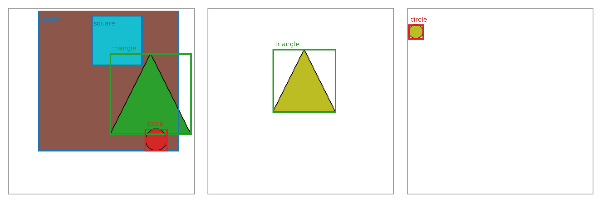
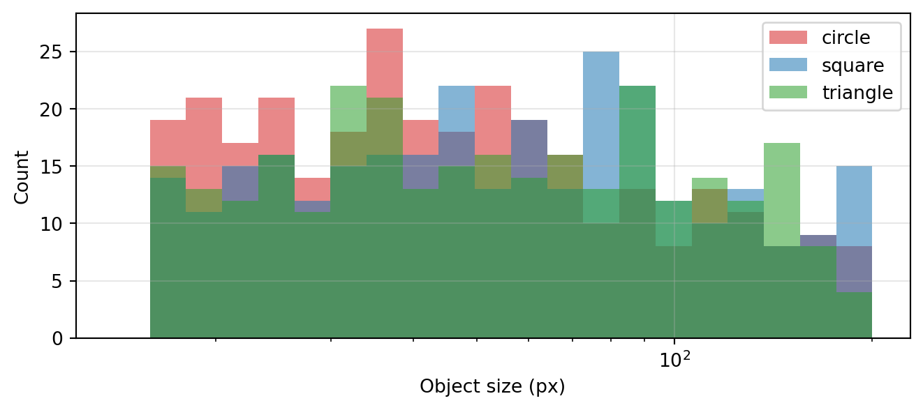
224×224 RGB images, 1–5 objects each. Three classes — circle, square, triangle — with object size drawn from the same range regardless of class. Boxes are \([x_1, y_1, x_2, y_2]\) in pixels.
One annotation record:
{
  "id": 0,
  "image_id": 0,
  "category_id": 1,
  "bbox": [
    37,
    4,
    205,
    172
  ]
}
Object sizes per class, over 300 training images:
Anchor Coverage
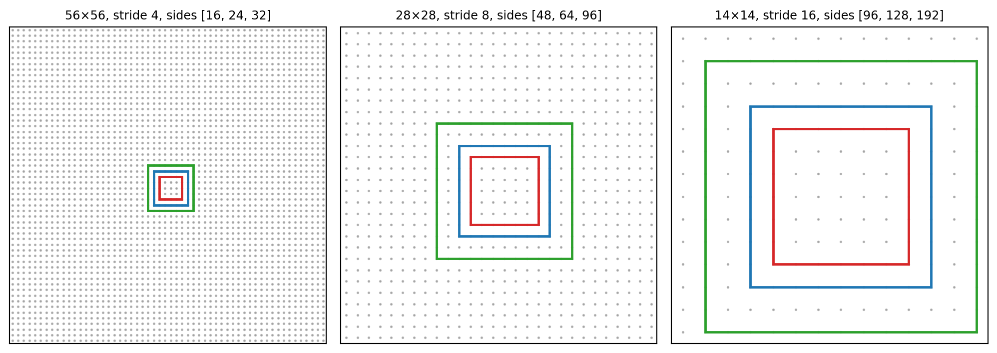
The three prediction scales tile the image at strides 4, 8, and 16, with three square anchors per cell. One cell’s anchors per scale, over the anchor-center grids:
Stick Figures
128×128 grayscale images, five keypoints per figure: head, left hand, right hand, left foot, right foot. Coordinates are \((x, y)\) in pixels.
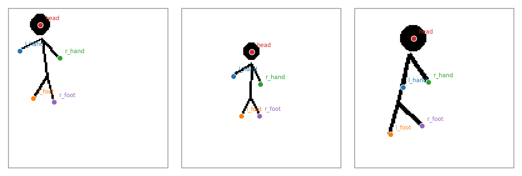
One annotation record:
{
  "id": 0,
  "image_id": 0,
  "keypoints": [
    [
      25.8,
      13.5
    ],
    [
      9.2,
      34.3
    ],
    [
      41.4,
      40.0
    ],
    [
      20.0,
      72.3
    ],
    [
      36.8,
      75.3
    ]
  ]
}
Heatmap Targets
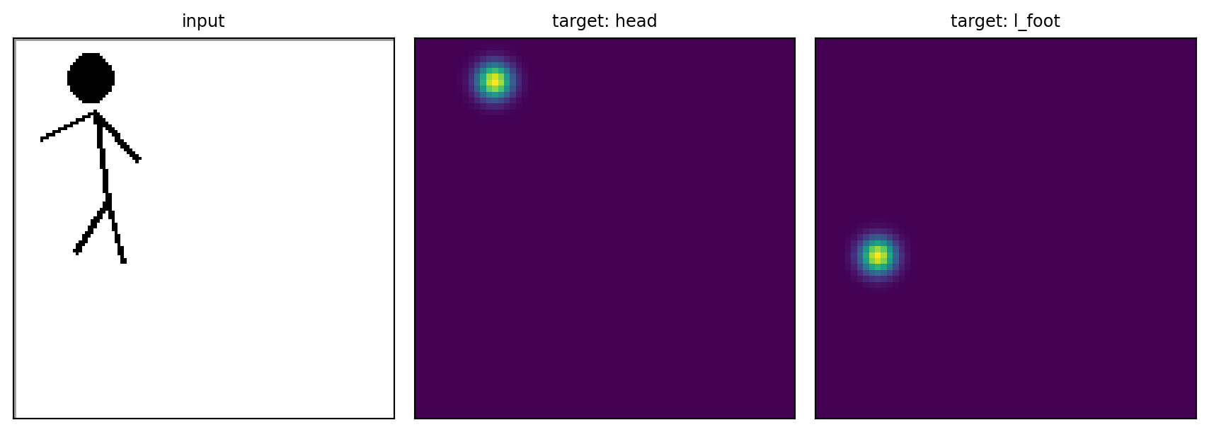
In heatmap mode, each keypoint becomes a 64×64 Gaussian target (\(\sigma = 2\) heatmap pixels, coordinates scaled by the heatmap/image ratio). One figure and two of its five targets:
Problem 1: Multi-Scale Single-Shot Detector
WarningRequirements
Implement everything yourself except the files under provided/ (NMS, average precision, visualization). Do not modify provided files.
Build a single-shot detector with three prediction scales. The core of the problem is turning sparse box annotations into a per-anchor training signal: anchor generation, matching, target encoding, and the multi-task loss.
Part A: Dataset
datasets/detection contains 224×224 RGB images with 1–5 shapes each. Object size is independent of class.
- Classes: 0 circle, 1 square, 2 triangle
- Annotations: JSON with boxes in \([x_1, y_1, x_2, y_2]\) pixel coordinates and class labels
Implement ShapeDetectionDataset and collate_fn in dataset.py. Images have a variable number of objects, so the collate function stacks images and keeps targets as a list of dicts.
Part B: Model
Implement MultiScaleDetector in model.py:
| Stage | Layers | Resolution |
|---|---|---|
| Stem | Conv(3→32, s1) → Conv(32→64, s2) | 224 → 112 |
| Block 2 | Conv(64→128, s2) | 112 → 56 → Scale 1 |
| Block 3 | Conv(128→256, s2) | 56 → 28 → Scale 2 |
| Block 4 | Conv(256→512, s2) | 28 → 14 → Scale 3 |
All convolutions are 3×3 with BatchNorm and ReLU. Each scale gets a detection head: two 3×3 convs (channels unchanged) followed by a 1×1 conv to num_anchors × (5 + num_classes) channels. The 5 is 4 box offsets \((t_x, t_y, t_w, t_h)\) plus 1 objectness logit.
Initialize the bias of each head’s objectness channels to \(-\log\frac{1 - \pi}{\pi}\) with \(\pi = 0.01\), so every anchor starts at objectness probability \(\approx 0.01\) rather than 0.5. With ~12,000 anchors and a few positives per image, background anchors starting at 0.5 dominate the early loss.
flatten_predictions reshapes the per-scale maps into one anchor-ordered tensor. The ordering is fixed: scales in order, row-major over each feature map (\(y\) outer, \(x\) inner), anchors within a cell. The interface tests check it.
Part C: Anchors, Matching, and Encoding
Implement anchors.py.
Anchors: square, centered at \(((x + 0.5) \cdot \text{stride}, (y + 0.5) \cdot \text{stride})\).
- Scale 1 (56×56): sides [16, 24, 32]
- Scale 2 (28×28): sides [48, 64, 96]
- Scale 3 (14×14): sides [96, 128, 192]
Encoding: targets are offsets relative to the matched anchor,
\[t_x = \frac{c_x - a_x}{a_w} \qquad t_y = \frac{c_y - a_y}{a_h} \qquad t_w = \log\frac{w}{a_w} \qquad t_h = \log\frac{h}{a_h}\]
where \((c_x, c_y, w, h)\) is the target box center/size and \((a_x, a_y, a_w, a_h)\) the anchor’s. decode_boxes inverts it.
Matching: concatenate the anchors of all three scales and match them jointly. An anchor is positive when its best IoU with any target is ≥ 0.5 and negative otherwise, with no ignore band, so near-miss anchors become hard-negative candidates. Force the highest-IoU anchor for each target positive so every target trains. Matched labels use 0 for background and class + 1 otherwise.
Part D: Loss
Implement DetectionLoss in loss.py:
- Objectness: binary cross-entropy on all positives plus mined negatives
- Classification: cross-entropy over the 3 classes, positive anchors only
- Localization: Smooth L1 on encoded offsets, positive anchors only, weight 2.0
- Hard negative mining: keep the highest-loss negatives at 3× the positive count
- Normalize all three terms by the number of positive anchors
Part E: Training
Complete train.py. The configuration is fixed: SGD with momentum 0.9, learning rate 0.01 stepped ×0.1 at epoch 40, batch size 16, 50 epochs. Save the best model by validation loss and log per-epoch losses to results/training_log.json.
Part F: Evaluation
Complete evaluate.py. The pipeline is fixed: score = sigmoid(objectness) × softmax(class), confidence filter at 0.05, per-class NMS at IoU 0.5 (provided), then AP per class (provided, all-point interpolation).
analyze_scale_specialization attributes each ground-truth object to the pyramid level that detected it (best-matching detection at IoU ≥ 0.5) and produces the size-vs-level histogram via the provided plotting helper.
Deliverables
See Submission.
results/metrics.jsonwith per-class AP, mAP, and matches per level.- Visualizations: detections on 10 validation images, the size-vs-level histogram, training curves.
- Report: which object sizes each scale detects, explained from the anchor configuration. The effect of the force-match rule on objects whose size falls between anchor bands. Where the detector fails, with examples.
Problem 2: Heatmap vs Direct Regression for Keypoints
WarningRequirements
Both networks must use the shared Encoder — the comparison isolates the output representation, so the feature extractor is identical by construction.
Localize 5 keypoints (head, hands, feet) on stick figures two ways: predict a spatial heatmap per keypoint, or regress coordinates directly. Same data, same encoder, same loss family. Measure the difference.
Part A: Dataset
datasets/keypoints contains 128×128 grayscale images with keypoint annotations in pixel coordinates. Implement KeypointDataset in dataset.py with two target modes:
'heatmap': one Gaussian per keypoint, rendered at 64×64. Keypoint coordinates scale by the heatmap/image ratio. Peak value ≈ 1.'regression': a flat \([10]\) vector of \((x, y)\) pairs normalized to \([0, 1]\) by the image size.
Gaussian sigma is a constructor parameter (default 2.0, in heatmap pixels).
Part B: Models
Implement model.py. The shared encoder:
| Stage | Layers | Resolution |
|---|---|---|
| Conv1 | Conv(1→32) → BN → ReLU → MaxPool | 128 → 64 |
| Conv2 | Conv(32→64) → BN → ReLU → MaxPool | 64 → 32 |
| Conv3 | Conv(64→128) → BN → ReLU → MaxPool | 32 → 16 |
| Conv4 | Conv(128→256) → BN → ReLU → MaxPool | 16 → 8 |
HeatmapNet decodes back to 64×64 with skip connections:
| Stage | Layers | Resolution |
|---|---|---|
| Deconv4 | ConvTranspose(256→128) → BN → ReLU | 8 → 16 |
| concat Conv3 skip → 256 channels | ||
| Deconv3 | ConvTranspose(256→64) → BN → ReLU | 16 → 32 |
| concat Conv2 skip → 128 channels | ||
| Deconv2 | ConvTranspose(128→32) → BN → ReLU | 32 → 64 |
| Head | Conv(32→5), no activation | 64 |
RegressionNet pools and regresses: global average pool → Linear(256→128) → ReLU → Dropout(0.5) → Linear(128→64) → ReLU → Dropout(0.5) → Linear(64→10) → Sigmoid.
Part C: Training
Complete train.py. Both models: MSE loss, Adam at lr 0.001, batch size 32, 30 epochs. Save best models by validation loss and log both training curves.
Part D: Evaluation
Complete evaluate.py:
extract_keypoints_from_heatmaps: argmax per heatmap, scaled back to image pixelscompute_pck: fraction of keypoints within a threshold distance of ground truth, normalized by the diagonal of the box enclosing the figure’s keypoints. Thresholds [0.05, 0.1, 0.15, 0.2]- PCK curves for both methods on one figure, and prediction visualizations for both methods
Part E: Sigma
Retrain the heatmap model with sigma 1.0 and 4.0 (train.py takes --sigma and --suffix). Evaluate PCK for all three sigmas.
Deliverables
See Submission.
results/pck_results.jsonwith PCK at all thresholds for both methods.- Visualizations: PCK comparison curves, sample predictions from both methods.
- Report: PCK for both methods at all thresholds and for the three sigma values. Compare the two representations and explain the result in terms of what the network must learn in each case. Address the spatial structure of the supervision and what global pooling discards. Which threshold regime separates the methods most, and why.
Submission Requirements
Your GitHub repository must follow this exact structure:
<repo>/
├── generate_datasets.py
├── q1/
│   ├── dataset.py
│   ├── model.py
│   ├── anchors.py
│   ├── loss.py
│   ├── train.py
│   ├── evaluate.py
│   ├── test_interfaces.py
│   ├── provided/
│   └── results/
│       ├── training_log.json
│       ├── metrics.json
│       └── visualizations/
├── q2/
│   ├── dataset.py
│   ├── model.py
│   ├── train.py
│   ├── evaluate.py
│   ├── test_interfaces.py
│   └── results/
│       ├── training_log.json
│       ├── pck_results.json
│       └── visualizations/
├── report/
│   └── report.pdf
└── README.md
Do not commit datasets/ or model weights — the starter’s .gitignore excludes both. report/report.tex is an optional LaTeX template for the report: one section per problem, deliverable items in order, figures embedded.
The README.md in your repository root contains your full name and student ID. See the submission guide for its full contents.
TipTesting Your Submission
Before submitting:
- Your repository structure must match the requirement exactly
python -m pytest test_interfaces.pymust pass in both problem directoriespython train.pyandpython evaluate.pymust run without errors in each problem directory- All output files must be generated in the correct locations