Homework #4: Reinforcement Learning

EE 641: Fall 2025

Assignment Details

Assigned: 12 November
Due: Tuesday, 25 November at 23:59

Submission: Gradescope via GitHub repository

Requirements

PyTorch >= 2.0 must be installed
Allowed libraries: PyTorch, NumPy, matplotlib, and Python standard library
No external RL libraries permitted (no Gymnasium, Stable Baselines, etc.)

Assignment Overview

In this assignment you will implement reinforcement learning algorithms through dynamic programming and deep Q-learning. The first problem implements Value Iteration and Q-Iteration to solve a stochastic gridworld navigation task. The second problem extends to multi-agent coordination where two agents learn to communicate and coordinate through DQN.

Getting Started

Download the starter code: hw4-starter.zip

Extract the starter code:

unzip hw4-starter.zip
cd hw4-starter

Submission Requirements

Your GitHub repository must follow this exact structure:

ee641-hw4-[username]/
├── problem1/
│   ├── environment.py
│   ├── value_iteration.py
│   ├── q_iteration.py
│   ├── train.py
│   ├── visualize.py
│   └── results/
│       └── visualizations/
├── problem2/
│   ├── multi_agent_env.py
│   ├── models.py
│   ├── replay_buffer.py
│   ├── train.py
│   ├── evaluate.py
│   └── results/
│       ├── agent_models/
│       ├── training_logs/
│       └── evaluation_results/
├── report.pdf
└── README.md

The README.md in your repository root must contain:

Your full name
USC email address
Instructions to run each problem if they differ from the standard commands
Any implementation notes

Testing Your Submission

Before submitting:

Your repository structure must match the requirement exactly
python train.py must run without errors in each problem directory
All output files must be generated in the correct locations
Test scripts should pass for interface compliance

Value and Q-Iteration on Stochastic Gridworld

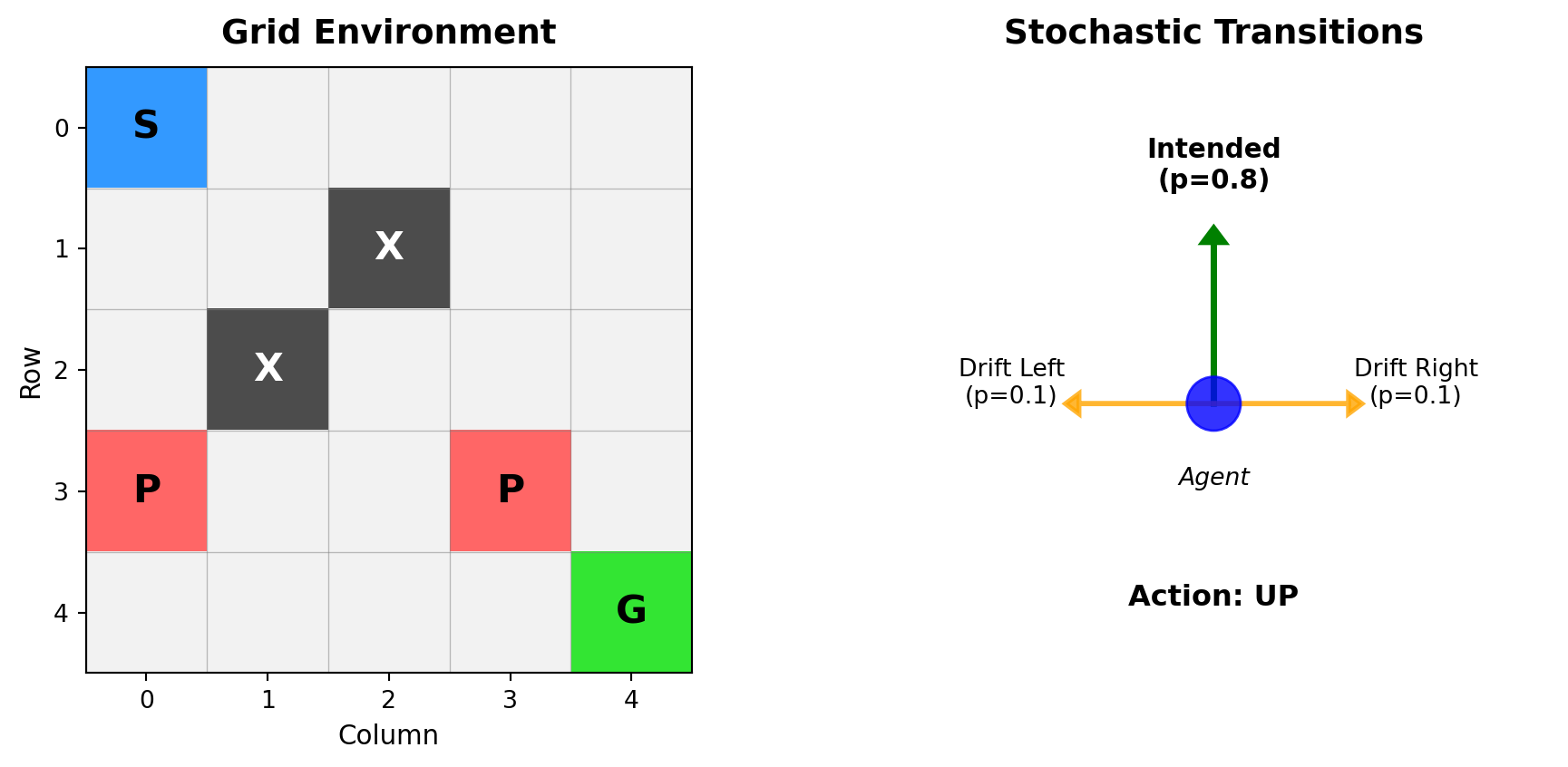
Implement Value Iteration and Q-Iteration to solve a stochastic gridworld navigation problem. A rescue robot must reach a goal location while navigating hazardous terrain with uncertain movement dynamics.

Environment Dynamics

The robot operates in a 5×5 grid with stochastic transitions:

0.8 probability: Move in intended direction
0.1 probability: Drift perpendicular left
0.1 probability: Drift perpendicular right

Collision with boundaries or obstacles results in no movement. The environment provides sparse rewards—most transitions incur small negative cost, while specific cells yield large positive or negative rewards upon entry.

Environment:

Goal (G): +10 reward, terminates episode
Penalty (P): -5 reward
Obstacles (X): Impassable cells
Regular movement: -0.1 cost per step

Parameters:

Episode limit: 50 steps maximum

Dynamic Programming Framework

Value Iteration operates in state space while Q-Iteration operates in state-action space.

Value Iteration

The optimal state-value function \(V^*(s)\) is the maximum expected return from state \(s\):

\[V^*(s) = \max_{a \in \mathcal{A}} \sum_{s' \in \mathcal{S}} P(s'|s,a) \left[ R(s,a,s') + \gamma V^*(s') \right]\]

The update rule:

\[V_{k+1}(s) \leftarrow \max_{a} \mathbb{E}_{s' \sim P(\cdot|s,a)} \left[ R(s,a,s') + \gamma V_k(s') \right]\]

Convergence is guaranteed for \(\gamma < 1\).

Q-Iteration

The action-value function \(Q^*(s,a)\) is the expected return when taking action \(a\) in state \(s\) then following the optimal policy:

\[Q^*(s,a) = \sum_{s'} P(s'|s,a) \left[ R(s,a,s') + \gamma \max_{a'} Q^*(s',a') \right]\]

Policy extraction: \(\pi^*(s) = \arg\max_a Q^*(s,a)\)

Update rule: \[Q_{k+1}(s,a) \leftarrow \sum_{s'} P(s'|s,a) \left[ R(s,a,s') + \gamma \max_{a'} Q_k(s',a') \right]\]

Implementation Details

For each state-action pair, consider all possible next states weighted by transition probabilities. With action \(a = \text{UP}\):

\(P(s_{\text{north}}|s, \text{UP}) = 0.8\) (intended)
\(P(s_{\text{west}}|s, \text{UP}) = 0.1\) (drift left)
\(P(s_{\text{east}}|s, \text{UP}) = 0.1\) (drift right)

If a transition would hit a wall or obstacle, the agent stays in the current state.

Convergence criterion: \[\|V_{k+1} - V_k\|_\infty = \max_{s \in \mathcal{S}} |V_{k+1}(s) - V_k(s)| < \epsilon\]

Use \(\epsilon = 10^{-4}\).

Tasks

You may use the provided starter code. Use discount factor γ = 0.95.

Implement the gridworld environment in Python using only NumPy and the standard Python libraries
Implement Value Iteration to compute the optimal state-value function using the Bellman optimality equation
Implement Q-Iteration to compute the optimal state-action value function
Derive the optimal policy from the computed value functions
Visualize the resulting optimal value function and policy on the grid. Display the value of each cell using a heatmap, and overlay arrows indicating the optimal action in each cell

Report Requirements

Your report for Problem 1 should include:

Number of iterations until convergence for both algorithms
Visualization of the final value function (heatmap)
Visualization of the optimal policy (arrows on grid)
Brief comparison of Value Iteration vs Q-Iteration convergence rates
Discussion of how the stochastic transitions affect the optimal policy

Multi-Agent Coordination with Limited Information

In multi-agent systems with partial observability, agents must coordinate using limited information. This problem examines what information enables coordination through systematic ablation of available signals.

Problem Setting

Two agents navigate a 10×10 gridworld with partial observability, attempting to simultaneously occupy a target location. Each agent observes only a 3×3 local patch centered on its position. Additional information channels may include distance to target and inter-agent communication.

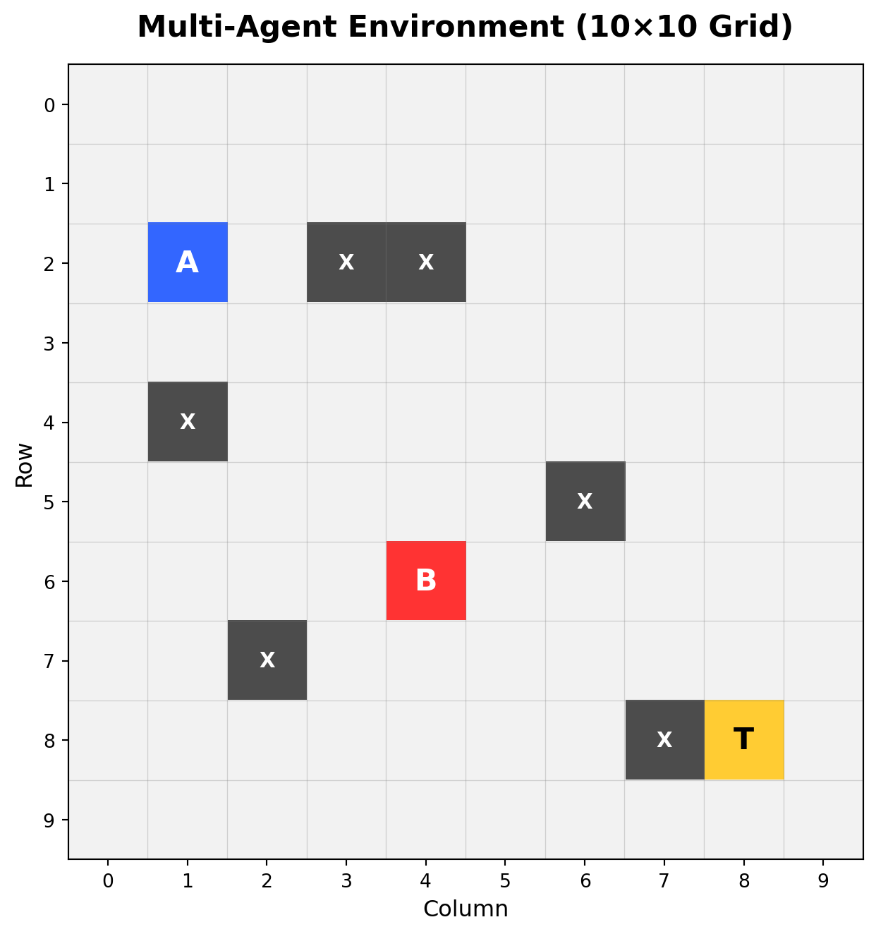
Environment:

Agents A and B: Must coordinate to reach target simultaneously
Target (T): Shared goal location
Obstacles (X): Impassable cells
Grid size: 10×10
Episode limit: 50 steps maximum

Observation and Action Spaces

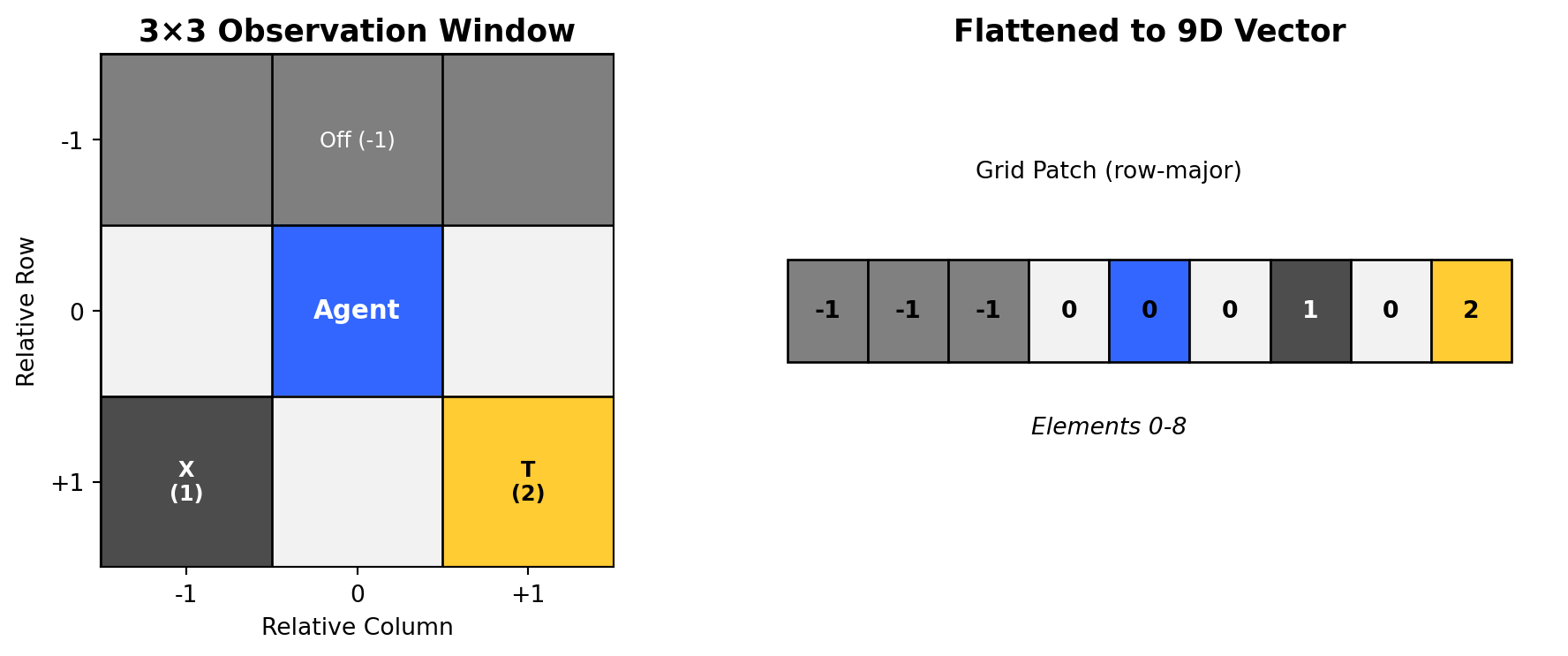
Base Scenario: Independent Agents

Each agent receives a 9-dimensional observation vector:

Elements 0-8: Flattened 3×3 grid patch (row-major order)
- Cell values: 0 (free), 1 (obstacle), 2 (target), -1 (off-grid)
- Agent positions not explicitly marked in observations

In this scenario, agents operate independently with only local observations.

Scenario B: Communication Channel

Observation extends to 10 dimensions:

Elements 0-8: Same as base scenario
Element 9: Communication scalar from partner agent (bounded [0,1])

Agents can now share information through a learned communication protocol.

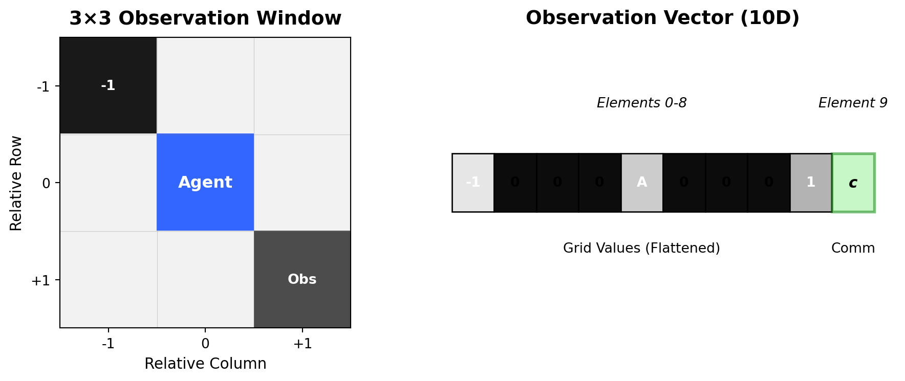
Scenario C: Distance and Communication

Observation extends to 11 dimensions:

Elements 0-8: Same as base scenario
Element 9: Communication scalar from partner agent
Element 10: Normalized distance between agents

Distance computation: \[d = \frac{\sqrt{(x_A - x_B)^2 + (y_A - y_B)^2}}{\sqrt{H^2 + W^2}}\]

where \((x_A, y_A)\) and \((x_B, y_B)\) are the positions of agents A and B, and \(H, W\) are grid dimensions. This distance represents signal strength in a beacon-like communication system. Normalization ensures the distance is bounded in [0,1] regardless of grid size, maintaining consistent input scale across different environments.

The action space combines movement and communication:

Movement actions: {Up, Down, Left, Right, Stay}
Communication output: Bounded scalar \(c \in [0, 1]\)

Deep Q-Network Architecture

The agent network processes partial observations to produce action-values and communication signals:

\[\begin{aligned} h &= \text{ReLU}(W_1 \cdot [\text{obs}, \text{comm}_{in}] + b_1) \\ Q(s,a) &= W_{action} \cdot h + b_{action} \quad \in \mathbb{R}^5 \\ c_{out} &= \sigma(W_{comm} \cdot h + b_{comm}) \quad \in [0, 1] \end{aligned}\]

Multi-Agent Q-Learning

The agents learn through independent Q-learning with shared experiences. The temporal difference target for agent \(i\):

\[y_i = r + \gamma \max_{a'} Q_i(s', a'; \theta^-_i)\]

where \(\theta^-\) represents target network parameters (updated periodically for stability). The loss combines both agents’ TD errors:

\[\mathcal{L} = \mathbb{E}_{(s,a,r,s') \sim \mathcal{D}} \left[ (Q_A(s_A, a_A) - y_A)^2 + (Q_B(s_B, a_B) - y_B)^2 \right]\]

Experience replay \(\mathcal{D}\) stores tuples \((s_A, s_B, a_A, a_B, c_A, c_B, r, s'_A, s'_B)\) capturing joint experiences.

Reward Structure

Reward structure:

\[R(s,a) = \begin{cases} +10 & \text{if both agents on target} \\ +2 & \text{if one agent on target} \\ -0.1 & \text{step penalty} \end{cases}\]

The partial reward for single-agent arrival provides intermediate feedback to guide exploration, while the full reward requires coordination.

Agents must:

Discover the target location through exploration
Coordinate arrival timing
Learn which actions and communications led to success

Tasks

You may use the provided starter code, but must follow the interfaces exactly. Use discount factor γ = 0.99.

Implement the multi-agent environment following the MultiAgentEnv interface specification below
Implement the DQN architecture with dual outputs (Q-values and communication signal) following the AgentDQN interface
Implement experience replay with batched updates
Implement \(\epsilon\)-greedy exploration for action selection
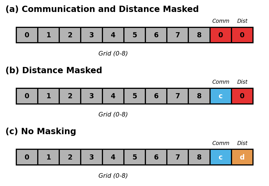
Conduct ablation study using a unified 11-dimensional observation space and single network architecture. Control information availability through input masking:
- (a) Independent: Mask elements 9-10 with zeros
- (b) Communication Only: Mask element 10 with zero
- (c) Full Information: No masking

Train all three configurations and save models in TorchScript format

Report Requirements

Your report for Problem 2 should include:

Training hyperparameters (learning rate, batch size, epsilon schedule, replay buffer size)
Training curves for all three configurations showing average reward and success rate
Final success rates for each configuration
Comparison table of performance across configurations
Analysis of how distance information and communication affect coordination
Discussion of learned strategies in each configuration

Required Interfaces

The following interfaces must be implemented exactly as specified for autograding:

Environment Interface

class MultiAgentEnv:
    def __init__(self, grid_size=(10, 10), obs_window=3, max_steps=50):
        """
        Initialize the environment.

        Parameters:
            grid_size: Tuple defining grid dimensions (default 10x10)
            obs_window: Size of local observation window (must be odd, default 3)
            max_steps: Maximum steps per episode
        """

    def reset(self):
        """
        Reset environment to initial state.

        Returns:
            obs_A, obs_B: Tuple[np.ndarray, np.ndarray]
            Each observation is an 11-dimensional vector:
            - Elements 0-8: Flattened 3x3 grid patch (row-major order)
            - Element 9: Communication signal from partner
            - Element 10: Normalized L2 distance between agents
        """

    def step(self, action_A, action_B, comm_A, comm_B):
        """
        Take a step in the environment.

        Parameters:
            action_A, action_B: Discrete actions (0:Up, 1:Down, 2:Left, 3:Right, 4:Stay)
            comm_A, comm_B: Communication scalars from each agent

        Returns:
            (obs_A, obs_B), reward, done
            - reward: +10 if both agents at target, +2 if one agent at target, -0.1 per step
            - done: True if both agents at target or max steps reached
        """

Network Interface

class AgentDQN(nn.Module):
    def __init__(self, input_dim=11, hidden_dim=64, num_actions=5):
        """
        Initialize the DQN.

        Parameters:
            input_dim: Dimension of input vector (default 11)
            hidden_dim: Number of hidden units (default 64)
            num_actions: Number of discrete actions (default 5)
        """

    def forward(self, x):
        """
        Forward pass.

        Parameters:
            x: Tensor of shape [batch_size, input_dim]

        Returns:
            action_values: Tensor of shape [batch_size, num_actions]
            comm_signal: Tensor of shape [batch_size, 1]
        """