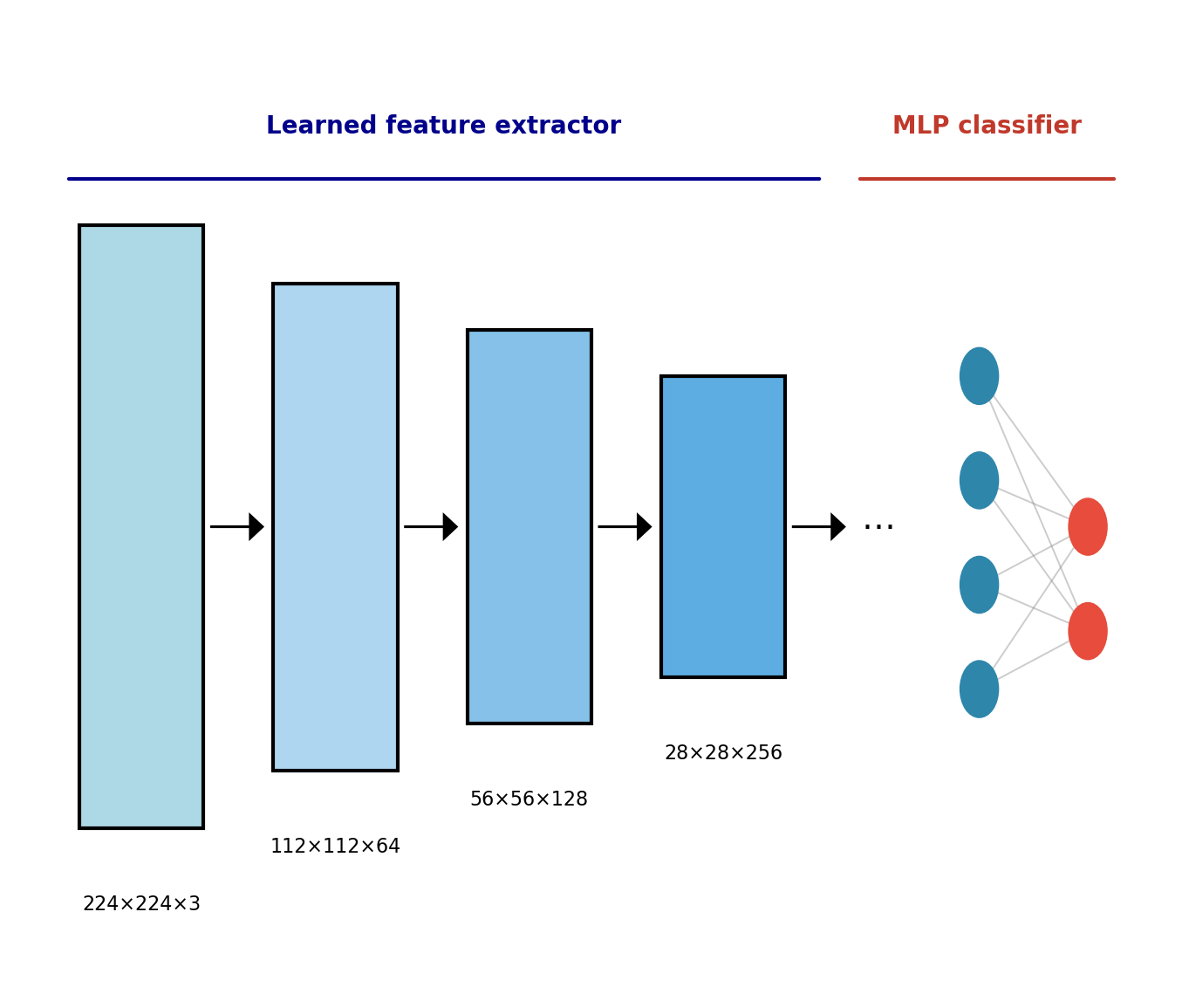
Advanced CNN Architectures
EE 641 - Unit 1
Convolution Is a Sliding Dot Product
Definition
For 2D discrete signals \(x\) and kernel \(h\):
\[(x * h)[i,j] = \sum_{m=0}^{K-1} \sum_{n=0}^{K-1} h[m,n] \cdot x[i+m, j+n]\]
where \(K\) is the kernel dimension.
Neural Network Convention
CNNs implement cross-correlation (not convolution):
- No kernel flipping
- Direct sliding dot product
- Mathematically: \((x \star h)\) not \((x * h)\)
This distinction is academic during learning since kernels are learned.
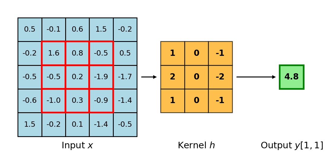
One output element requires \(K^2\) multiply–accumulate operations (MACs: one multiply, one add — 2 FLOPs)
Weight Sharing Removes Input Size from the Parameter Count
Dense layer: parameters scale with activation counts
\[N_{\text{in}} \times N_{\text{out}}\]
Convolutional layer: parameters scale with kernel and channels only
\[K^2 \cdot C_{\text{in}} \cdot C_{\text{out}} + C_{\text{out}} \quad \text{— independent of } H \times W\]
Worked Example
nn.Conv2d(16, 32, kernel_size=3, padding=1) on 64×64 input:
| Quantity | Size |
|---|---|
| Input activations | 16×64×64 = 65,536 |
| Output activations | 32×64×64 = 131,072 |
| Filter weights | 32×(3×3×16) = 4,608 |
| Biases | 32 |
| Trainable parameters | 4,640 |
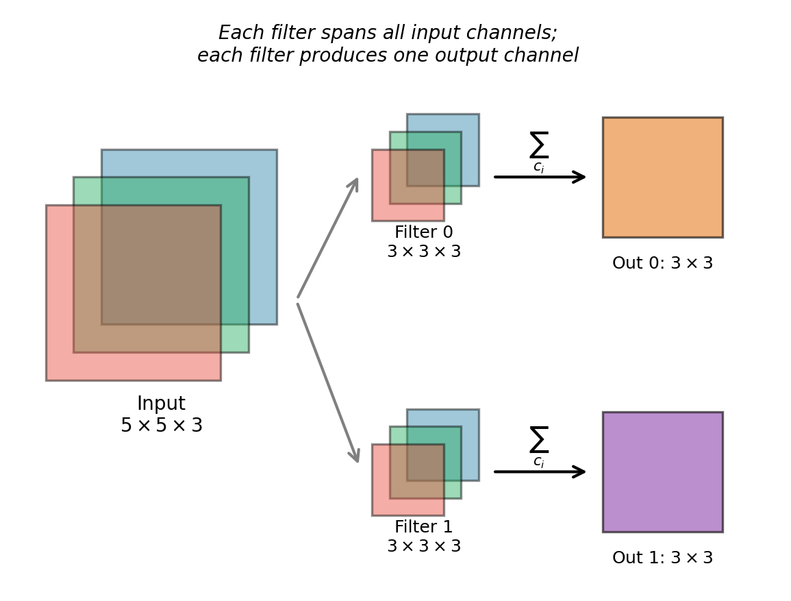
Each filter spans the full input depth: 3×3×16.
Dense layer with the same activations: \(65{,}536 \times 131{,}072 + 131{,}072 \approx 8.59 \times 10^9\) — a 1.85 million× reduction.
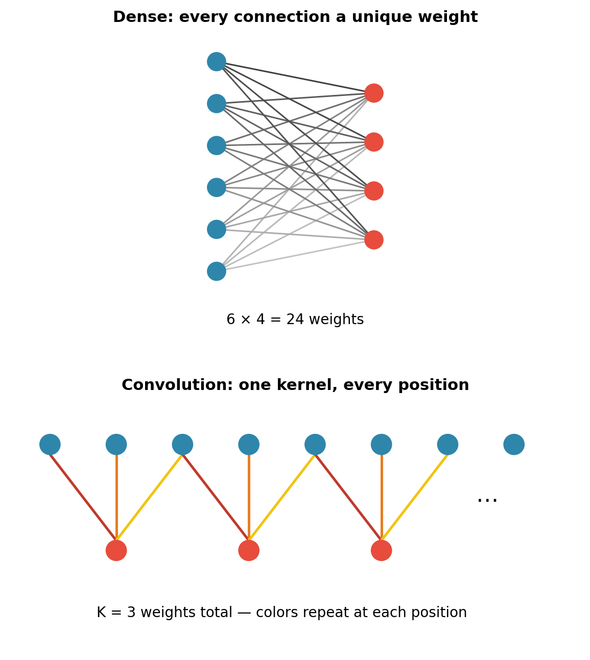
Trade off: fewer parameters, more computation per parameter — 4,640 weights perform 18.9M MACs, each weight applied at all 4,096 spatial positions.
The Transpose Reverses the Forward Pass
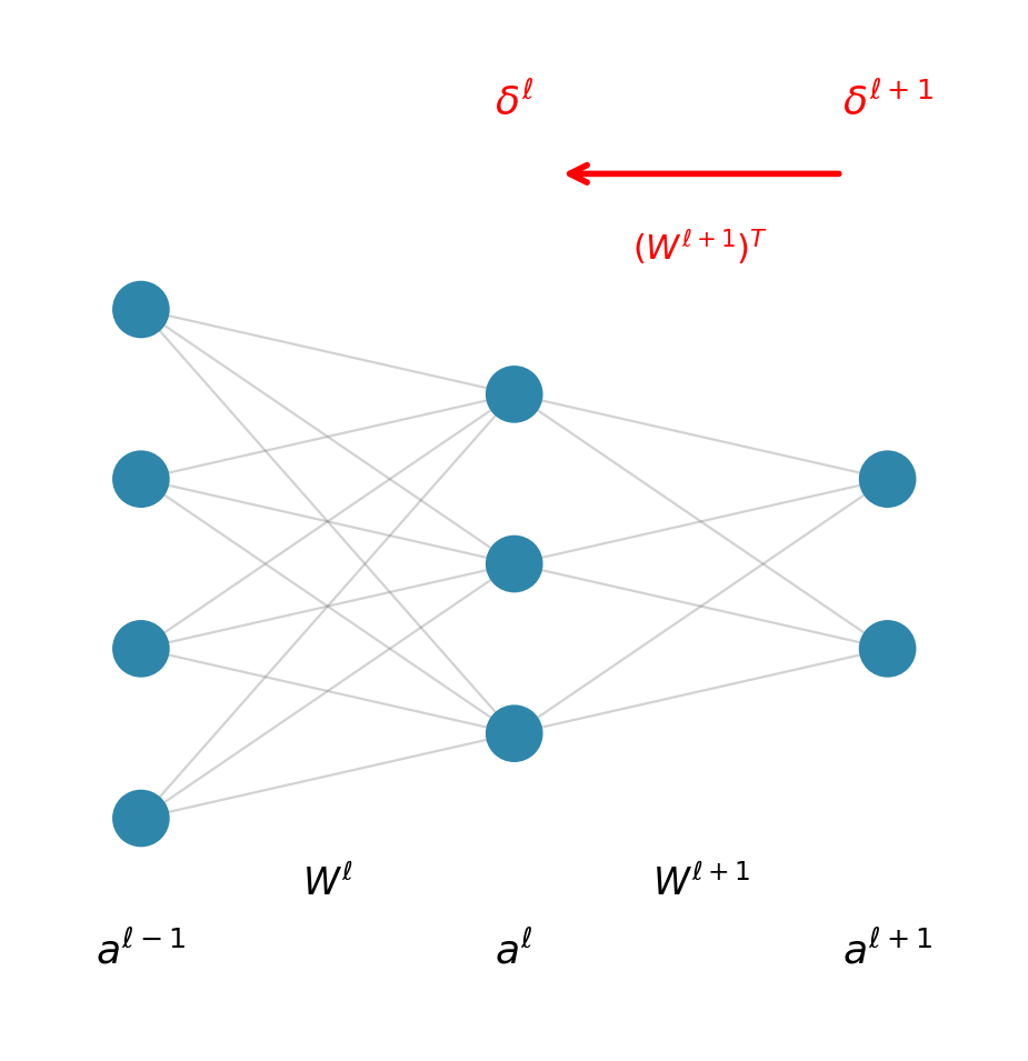
For layer \(\ell\) with pre-activation \(z^\ell = W^\ell a^{\ell-1} + b^\ell\):
\[\delta^\ell = \frac{\partial \mathcal{L}}{\partial z^\ell} = (W^{\ell+1})^T \delta^{\ell+1} \odot \sigma'(z^\ell)\]
Weight gradient: \[\frac{\partial \mathcal{L}}{\partial W^\ell_{ij}} = \delta^\ell_i \cdot a^{\ell-1}_j\]
Matrix form: \[\frac{\partial \mathcal{L}}{\partial W^\ell} = \delta^\ell (a^{\ell-1})^T\]
The transpose operation \((W^{\ell+1})^T\) reverses the linear transformation during backpropagation.
One Input Element Feeds a K×K Output Region
\[\text{Given } \underbrace{\frac{\partial \mathcal{L}}{\partial y[i,j]}}_{\delta^\ell \;(y \,=\, z^\ell)} \text{, we require } \underbrace{\frac{\partial \mathcal{L}}{\partial x[p,q]}}_{\delta^{\ell-1} \text{ after } \odot\, \sigma'}\]
Dependency Analysis
Element \(x[p,q]\) contributes to output positions: \[\{y[i,j] : p-K+1 \leq i \leq p, \; q-K+1 \leq j \leq q\}\]
By chain rule: \[\frac{\partial \mathcal{L}}{\partial x[p,q]} = \sum_{i,j} \frac{\partial \mathcal{L}}{\partial y[i,j]} \cdot \frac{\partial y[i,j]}{\partial x[p,q]}\]
Since \(y[i,j] = \sum_{m,n} h[m,n] \cdot x[i+m, j+n]\):
\[\frac{\partial y[i,j]}{\partial x[p,q]} = \begin{cases} h[p-i, q-j] & \text{if } 0 \leq p-i < K, \; 0 \leq q-j < K \\ 0 & \text{otherwise} \end{cases}\]
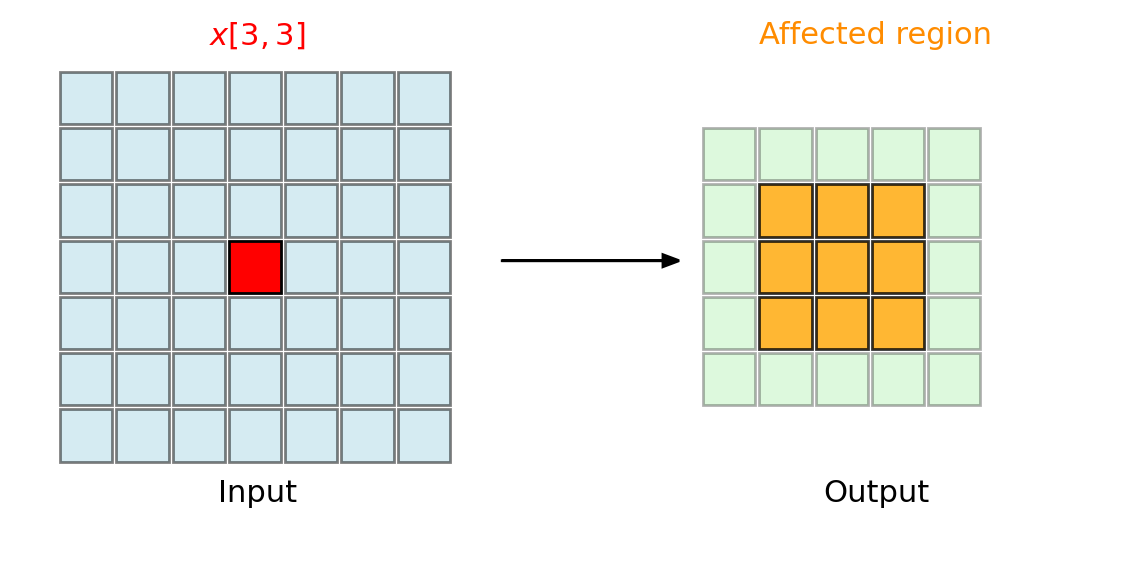
\(x[3,3]\) influences a \(3 \times 3\) region in output (for \(K=3\))
Transposed Convolution Emerges
Substituting the partial derivative:
\[\frac{\partial \mathcal{L}}{\partial x[p,q]} = \sum_{i=p-K+1}^{p} \sum_{j=q-K+1}^{q} \frac{\partial \mathcal{L}}{\partial y[i,j]} \cdot h[p-i, q-j]\]
Change of variables: \(m = p-i\), \(n = q-j\):
\[\frac{\partial \mathcal{L}}{\partial x[p,q]} = \sum_{m=0}^{K-1} \sum_{n=0}^{K-1} h[m,n] \cdot \frac{\partial \mathcal{L}}{\partial y[p-m, q-n]}\]
This is convolution with a rotated kernel:
\[\boxed{\frac{\partial \mathcal{L}}{\partial x} = \frac{\partial \mathcal{L}}{\partial y} * h^{\text{rot180}}}\]
where \(h^{\text{rot180}}[m,n] = h[K-1-m, K-1-n]\)
The conv form of \((W^\ell)^T \delta^\ell\) — kernel rotation is the transpose.
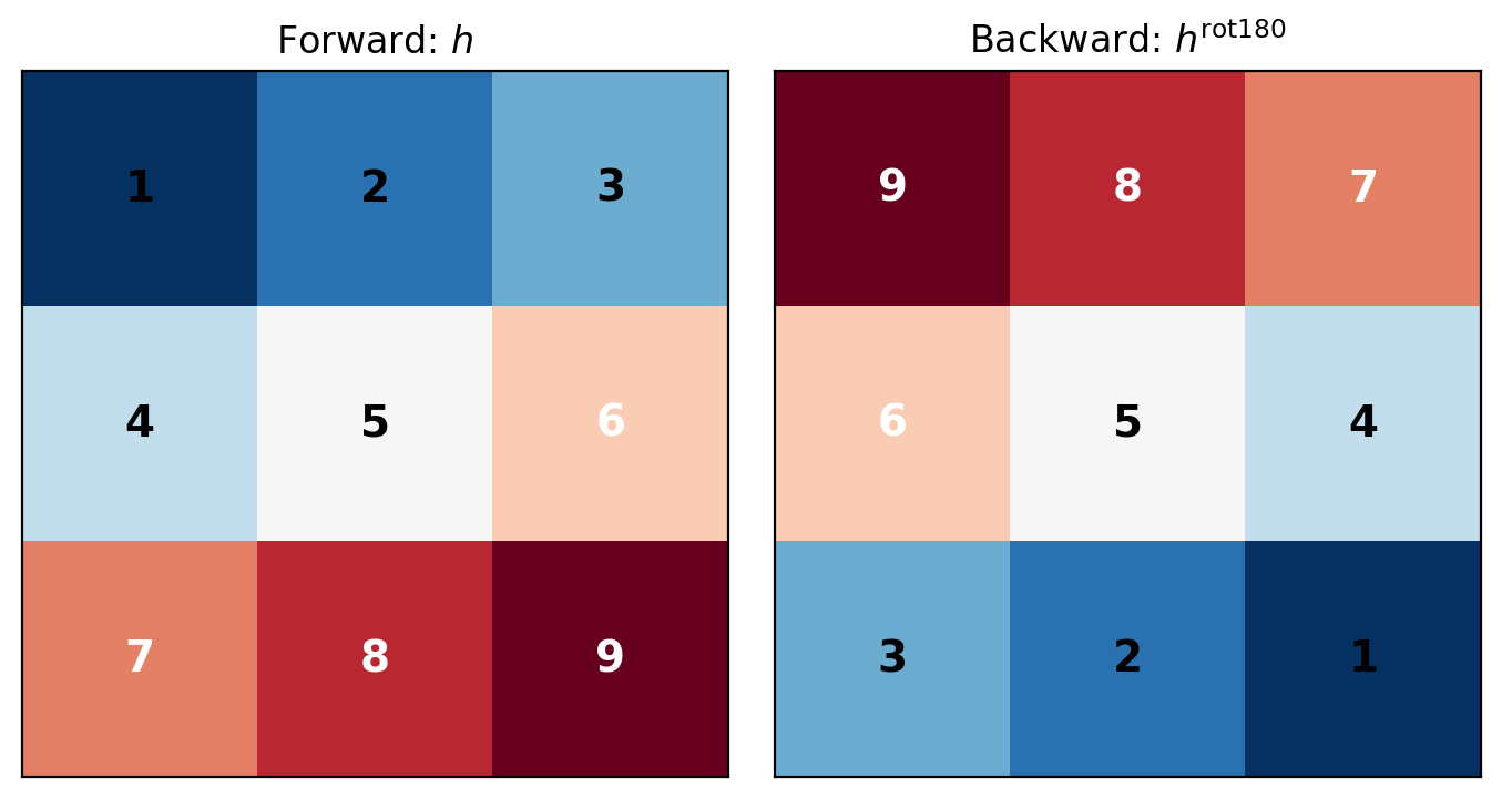
180° rotation: \(h[m,n] \rightarrow h[K-1-m, K-1-n]\)
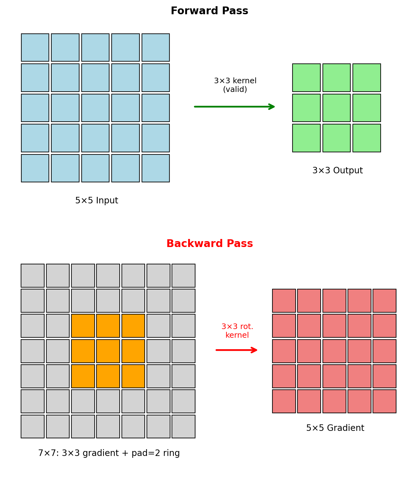
The Backward Pass Requires pad = K − 1
Forward Pass
- Input: \(H \times W\)
- Kernel: \(K \times K\)
- Valid convolution: \((H-K+1) \times (W-K+1)\)
Backward Pass
- Gradient w.r.t. output: \((H-K+1) \times (W-K+1)\)
- Need gradient w.r.t. input: \(H \times W\)
Required Padding
To recover original dimensions: \[\text{pad} = K - 1\]
This yields “full” convolution in backward pass.
Weight Gradients Are Input–Gradient Correlations
Derivation
Each kernel element \(h[m,n]\) appears in computing all output positions:
\[\frac{\partial \mathcal{L}}{\partial h[m,n]} = \sum_{i,j} \frac{\partial \mathcal{L}}{\partial y[i,j]} \cdot \frac{\partial y[i,j]}{\partial h[m,n]}\]
From \(y[i,j] = \sum_{m',n'} h[m',n'] \cdot x[i+m', j+n']\):
\[\frac{\partial y[i,j]}{\partial h[m,n]} = x[i+m, j+n]\]
Therefore: \[\boxed{\frac{\partial \mathcal{L}}{\partial h[m,n]} = \sum_{i,j} \frac{\partial \mathcal{L}}{\partial y[i,j]} \cdot x[i+m, j+n]}\]
This is the correlation between input and output gradient — the conv form of \(\delta^\ell (a^{\ell-1})^T\), the outer product summed over shared positions.
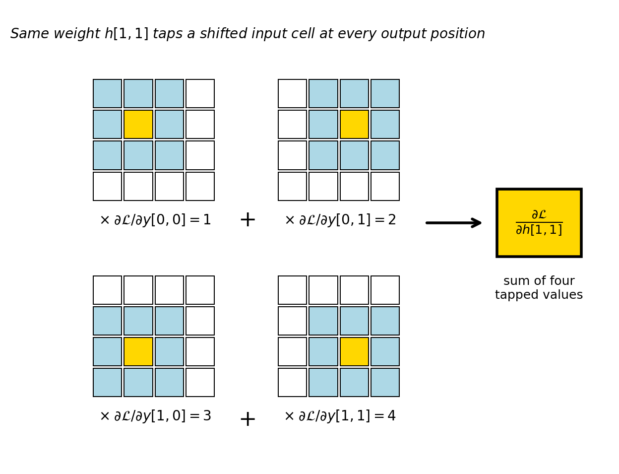
Each weight gradient accumulates contributions from all spatial positions where that weight was applied.
Stacked Small Kernels Build Large Receptive Fields
Receptive Field
Input region influencing one output element. For stacked stride-1 convolutions:
\[r = 1 + \sum_{\ell} (K_\ell - 1)\]
Two 3×3 layers: \(r = 5\). Three 3×3 layers: \(r = 7\).
Cost Comparison (C channels in and out)
| Configuration | Params | Same \(r\) as | Savings |
|---|---|---|---|
| Two 3×3 | \(18C^2\) | one 5×5 (\(25C^2\)) | 28% |
| Three 3×3 | \(27C^2\) | one 7×7 (\(49C^2\)) | 45% |
Plus one extra nonlinearity per layer.
VGG (2014) established the convention; \(K=3\) has been the default since.
Dilated kernels grow \(r\) without additional parameters — spacing \(d\) between taps gives effective extent \(d(K-1)+1\).
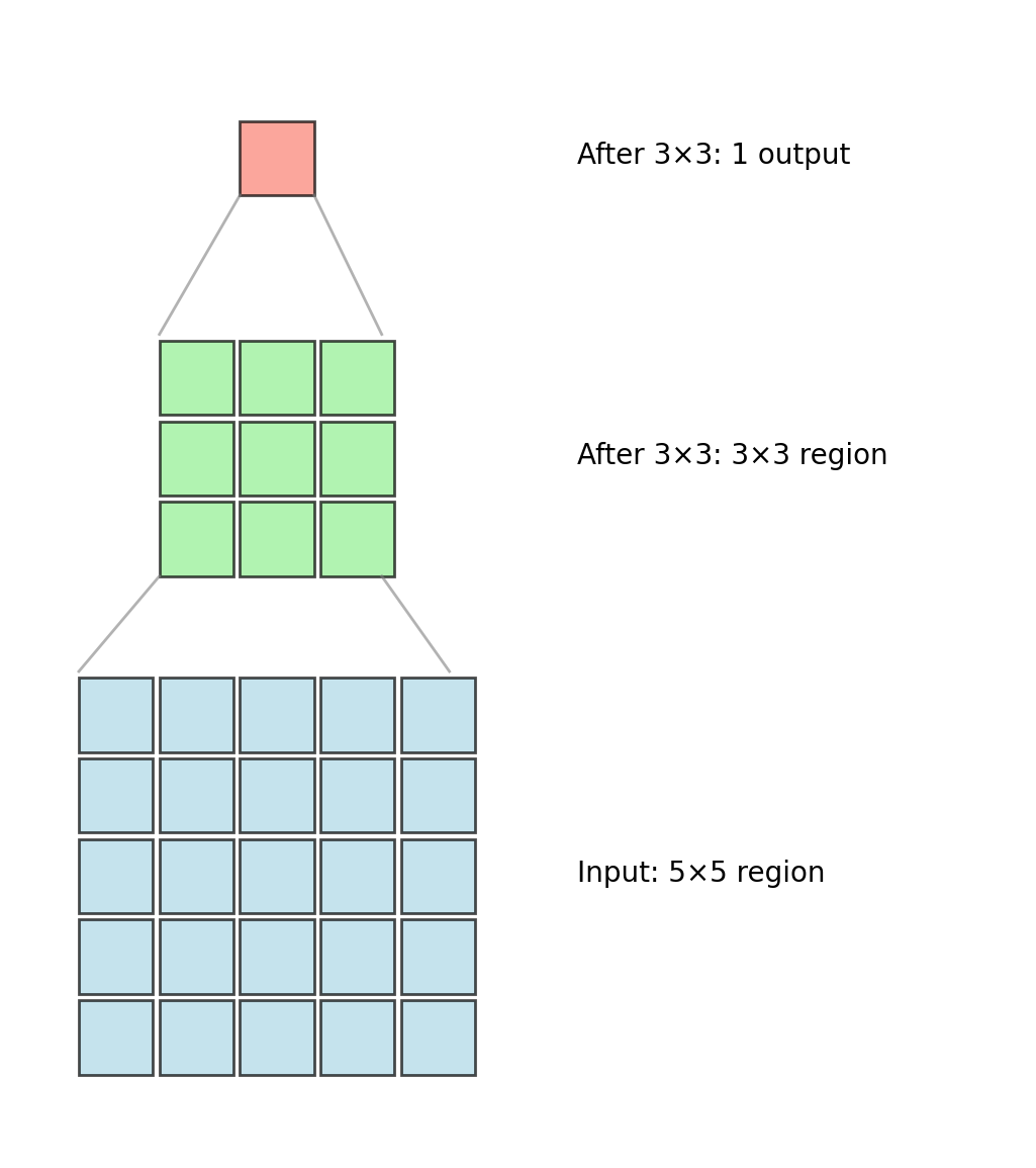
\(18C^2\) parameters see the same extent as \(25C^2\) — with two nonlinearities.
CNNs Trade Spatial Resolution for Channel Depth
The Stage Pattern
Several convolutions at fixed resolution, then downsample:
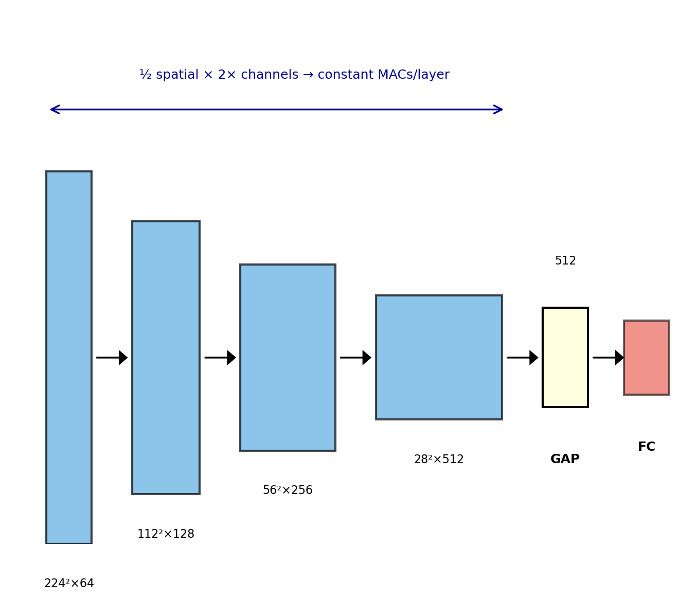
- Spatial: \(H, W \rightarrow H/2, W/2\)
- Channels: \(C \rightarrow 2C\)
Why This Ratio
Per-layer compute \(\propto H \cdot W \cdot K^2 \cdot C_{\text{in}} \cdot C_{\text{out}}\)
Halving spatial (÷4) while doubling channels (×4) → constant compute per layer across stages.
Each downsample also doubles the receptive-field growth rate of every subsequent layer — late stages see the entire image.
The Head
Global average pooling: \(H \times W \times C \rightarrow C\), any input size.
- VGG-16 FC head: 123.6M of 138.4M params (89%)
- ResNet-50 GAP head: 2.05M of 25.6M (8%)
Two downsampling mechanisms: strided convolution and pooling.
Stride Downsamples Forward, Dilates Backward
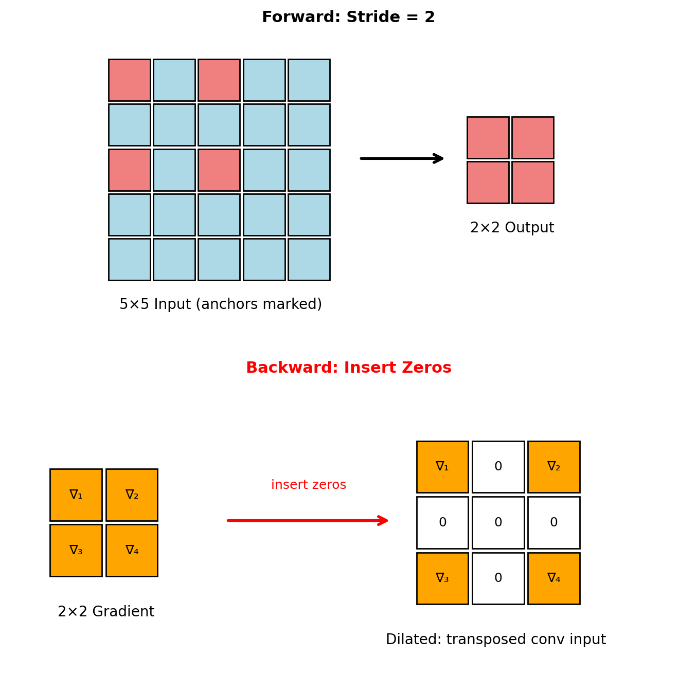
Forward (stride \(s > 1\))
Output dimension: \[H_{\text{out}} = \left\lfloor \frac{H_{\text{in}} - K}{s} \right\rfloor + 1\]
Convolution with stride \(s\): \[y[i,j] = \sum_{m,n} h[m,n] \cdot x[si+m, sj+n]\]
Backward (fractional stride)
Insert \((s-1)\) zeros between gradient elements: \[\tilde{g}[i,j] = \begin{cases} \frac{\partial \mathcal{L}}{\partial y[i/s, j/s]} & \text{if } s|i \text{ and } s|j \\ 0 & \text{otherwise} \end{cases}\]
Then apply standard transposed convolution to \(\tilde{g}\).
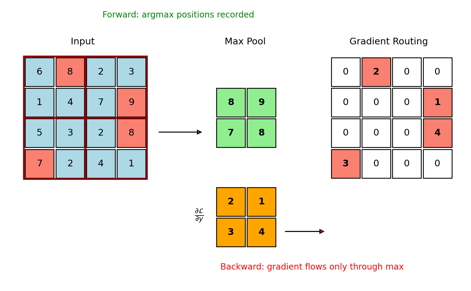
Max Pooling: Gradient Routing
Forward Sums Input Channels, Backward Sums Output Channels
Tensor Dimensions
- Input: \((H, W, C_{\text{in}})\)
- Kernels: \((K, K, C_{\text{in}}, C_{\text{out}})\)
- Output: \((H', W', C_{\text{out}})\)
Forward Computation
\[y[i,j,c_o] = \sum_{c_i=0}^{C_{\text{in}}-1} \sum_{m=0}^{K-1} \sum_{n=0}^{K-1} h[m,n,c_i,c_o] \cdot x[i+m,j+n,c_i]\]
Gradient Computation
Input gradient (sum over output channels): \[\frac{\partial \mathcal{L}}{\partial x[p,q,c_i]} = \sum_{c_o=0}^{C_{\text{out}}-1} \left( \frac{\partial \mathcal{L}}{\partial y[\cdot,\cdot,c_o]} * h^{\text{rot180}}[\cdot,\cdot,c_i,c_o] \right)[p,q]\]
Weight gradient (correlation structure): \[\frac{\partial \mathcal{L}}{\partial h[m,n,c_i,c_o]} = \sum_{i,j} \frac{\partial \mathcal{L}}{\partial y[i,j,c_o]} \cdot x[i+m,j+n,c_i]\]
The Vanishing Gradient Problem Revisited
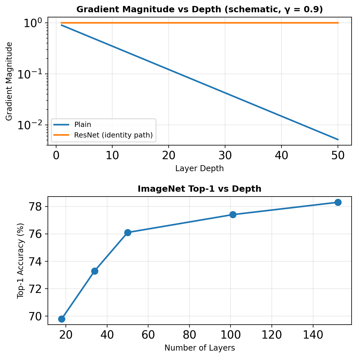
Gradient Magnitude Decay
For a network with \(L\) layers: \[\frac{\partial \mathcal{L}}{\partial x_1} = \prod_{\ell=1}^{L} \frac{\partial f_\ell}{\partial x_{\ell-1}}\]
If \(\left|\frac{\partial f_\ell}{\partial x_{\ell-1}}\right| < 1\): \[\left|\frac{\partial \mathcal{L}}{\partial x_1}\right| \approx \gamma^L \rightarrow 0\]
ResNet Solution
Skip connections: \(x_\ell = \mathcal{F}_\ell(x_{\ell-1}) + x_{\ell-1}\)
Returns diminish with depth. The original ResNet-1001 degrades on CIFAR-10. Pre-activation block ordering (He et al., 2016b) restores the gain.
Residual Blocks Learn Corrections to the Identity
Block output: identity plus a learned residual
\[x_\ell = \mathcal{F}_\ell(x_{\ell-1}) + x_{\ell-1}\]
\(\mathcal{F}\) learns the correction to \(x\), not the full mapping. Zero weights give identity — depth cannot hurt initialization.
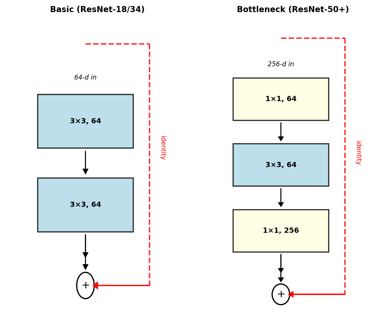
Basic block (ResNet-18/34): two 3×3 convs at full width.
Bottleneck block (ResNet-50+): 1×1 reduce → 3×3 → 1×1 restore.
The 3×3 runs at 64 channels inside 256-d input/output: basic-block cost (≈70K params) at 4× the width.
| Model | Params | GFLOPs | Top-1 |
|---|---|---|---|
| ResNet-18 | 11.7M | 1.8 | 69.8% |
| ResNet-34 | 21.8M | 3.7 | 73.3% |
| ResNet-50 | 25.6M | 4.1 | 76.1% |
| ResNet-101 | 44.5M | 7.8 | 77.4% |
| ResNet-152 | 60.2M | 11.5 | 78.3% |
Top-1: ImageNet validation accuracy — the highest-scoring class must be the labeled class.
Dimension changes (stride, channel growth) use a 1×1 projection on the shortcut.
Addition Can Wash Out Earlier Features
Additive Identity Mapping
Forward: \[x_\ell = \mathcal{F}_\ell(x_{\ell-1}) + x_{\ell-1}\]
Backward: \[\frac{\partial \mathcal{L}}{\partial x_{\ell-1}} = \frac{\partial \mathcal{L}}{\partial x_\ell} \left(1 + \frac{\partial \mathcal{F}_\ell}{\partial x_{\ell-1}}\right)\]
During training:
- Gradients split between paths
- Information “competition”
- Many paths contribute little
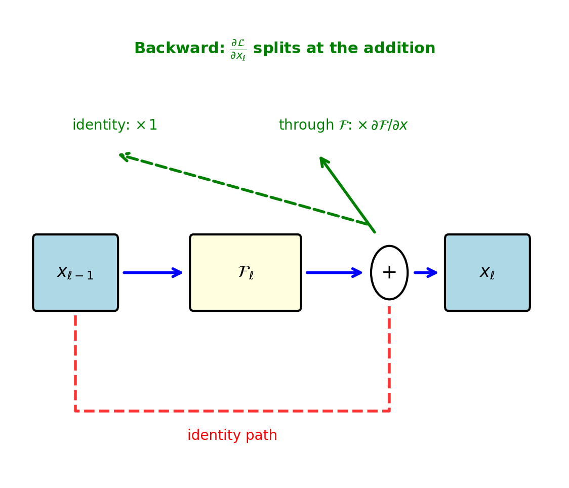
Addition can wash out earlier features
DenseNet Concatenates Instead of Adding
Concatenative Connections
Instead of addition: \[x_\ell = H_\ell([x_0, x_1, ..., x_{\ell-1}])\]
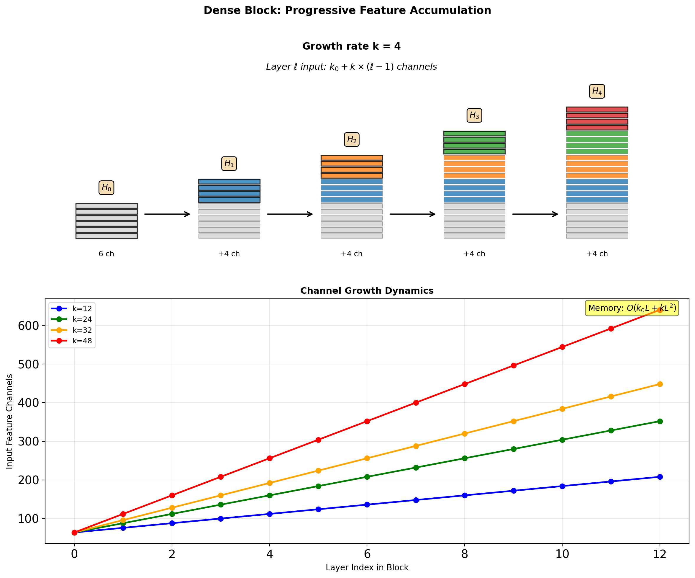
where \([\cdot]\) denotes concatenation and \(x_\ell\) is the \(k\) feature maps produced by layer \(\ell\) — the new slice, not a running state.
Direct connections: Layer \(\ell\) receives feature maps from all preceding layers
Gradient flow, with \(x_L\) the final layer’s output: \[\frac{\partial \mathcal{L}}{\partial x_i} = \frac{\partial \mathcal{L}}{\partial x_L} \frac{\partial x_L}{\partial x_i} + \sum_{j=i+1}^{L-1} \frac{\partial \mathcal{L}}{\partial x_j} \frac{\partial x_j}{\partial x_i}\]
\(L(L+1)/2\) connections in an \(L\)-layer network
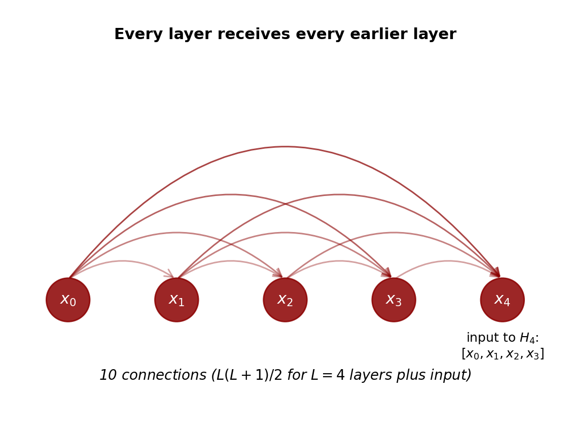
Each Layer Adds k Channels to a Growing Stack
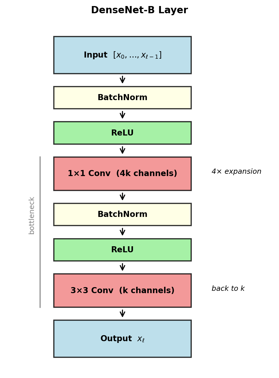
\(H_\ell\) Bottlenecks Through 4k Channels
Pre-activation Design
Standard DenseNet-B (Bottleneck):
- Batch Normalization
- ReLU
- 1×1 Convolution (4k channels)
- Batch Normalization
- ReLU
- 3×3 Convolution (k channels)
Pre-activation design rationale:
- Clean gradient path
- No need for careful initialization
- Identity mappings when needed
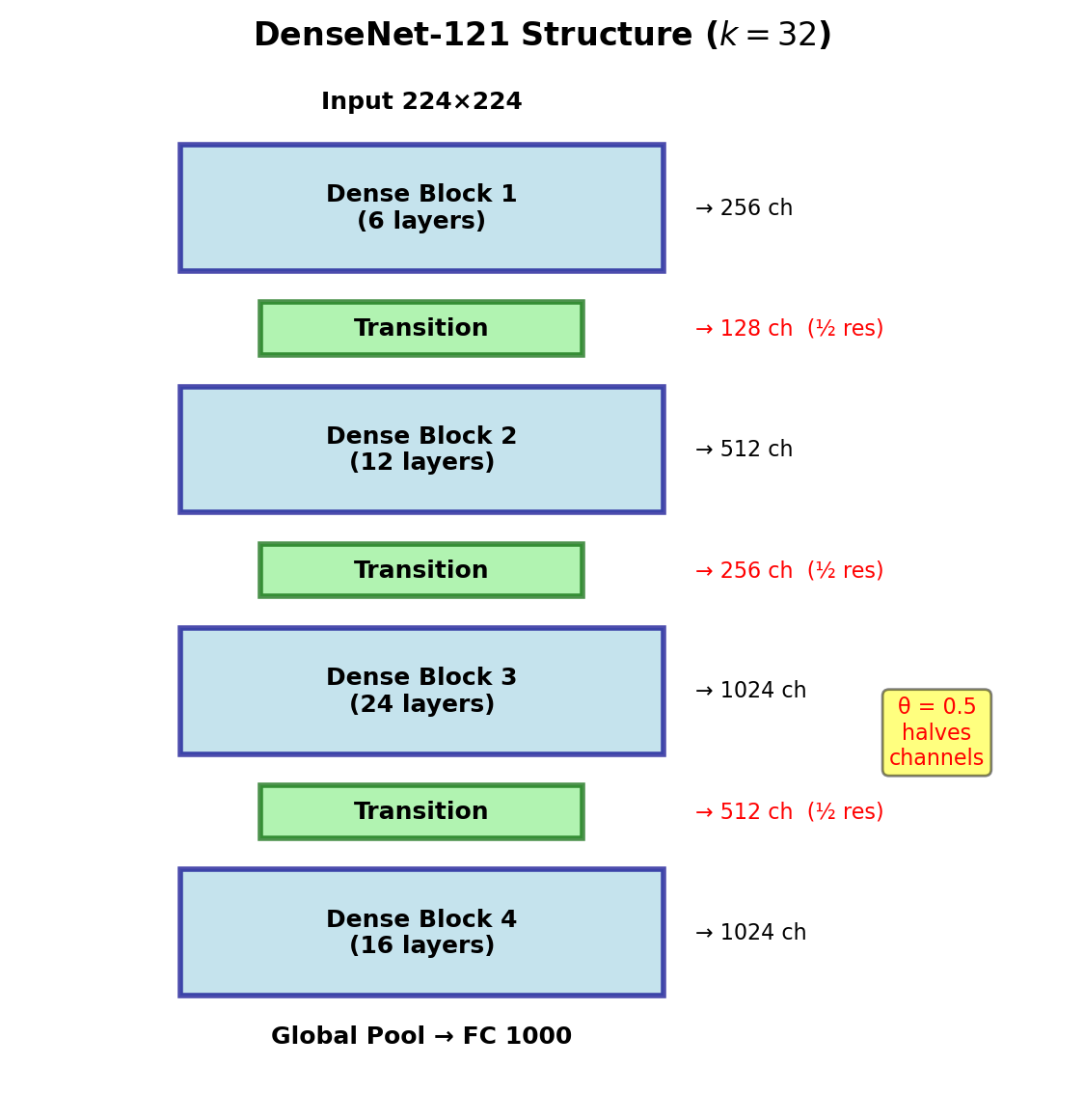
Transitions Halve Channels and Resolution
Between Dense Blocks
Purpose: Control model complexity
- Batch Normalization
- ReLU activation
- 1×1 Convolution
- 2×2 Average Pooling
Compression Factor \(\theta\)
If block outputs \(m\) feature maps:
- Transition reduces to \(\lfloor \theta m \rfloor\)
- DenseNet-C: \(\theta = 0.5\)
- DenseNet-BC: Bottleneck + Compression
Compression is critical for deep networks
The DenseNet Family: Accuracy per Parameter
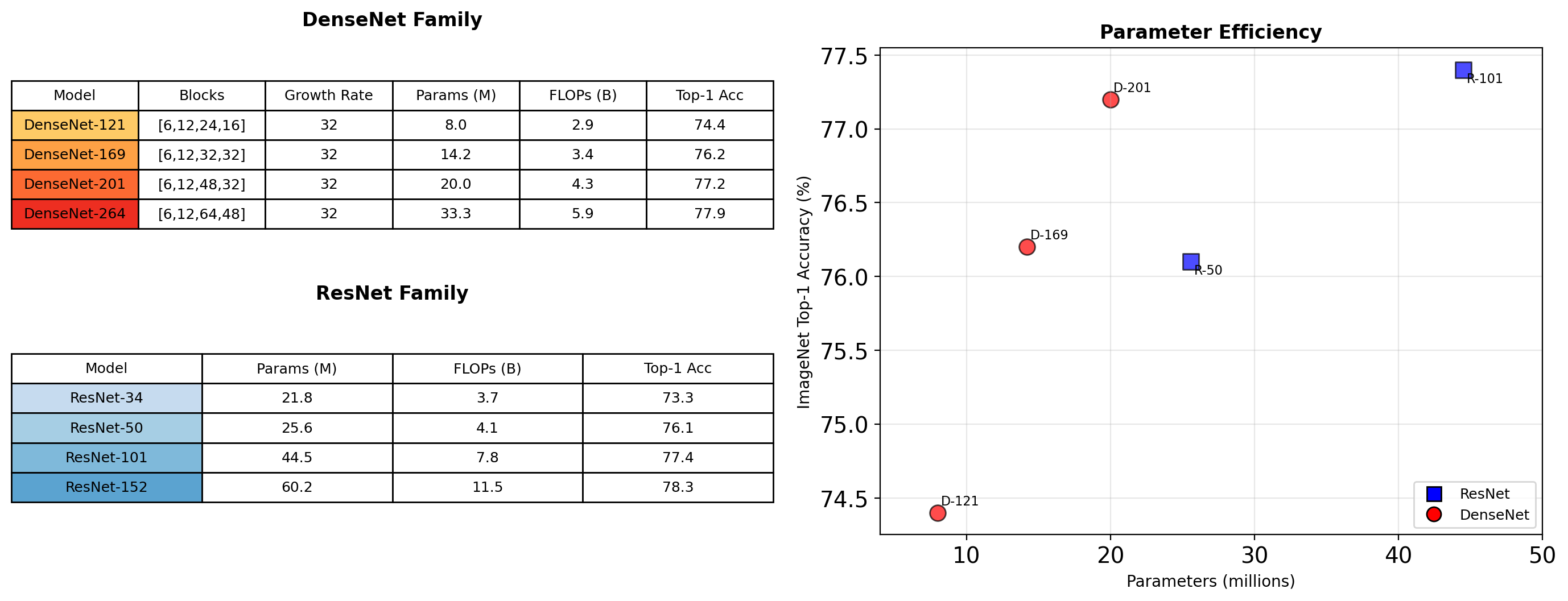
DenseNet-201 matches ResNet-101 accuracy at 2.2× fewer parameters
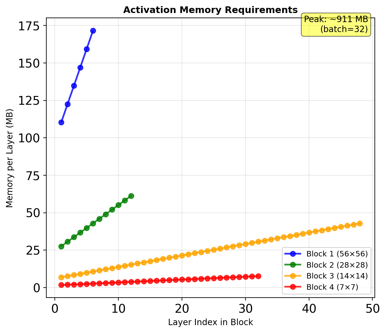
Concatenation Makes Activations the Memory Cost
Forward Pass Storage
Must maintain all intermediate features:
- Layer \(\ell\) needs: \([x_0, x_1, ..., x_{\ell-1}]\)
- Cannot free early activations
- Peak memory at block end
Implementation Strategy
Shared memory allocations:
Memory-efficient variant: Recompute activations during backward pass (trading compute for memory)
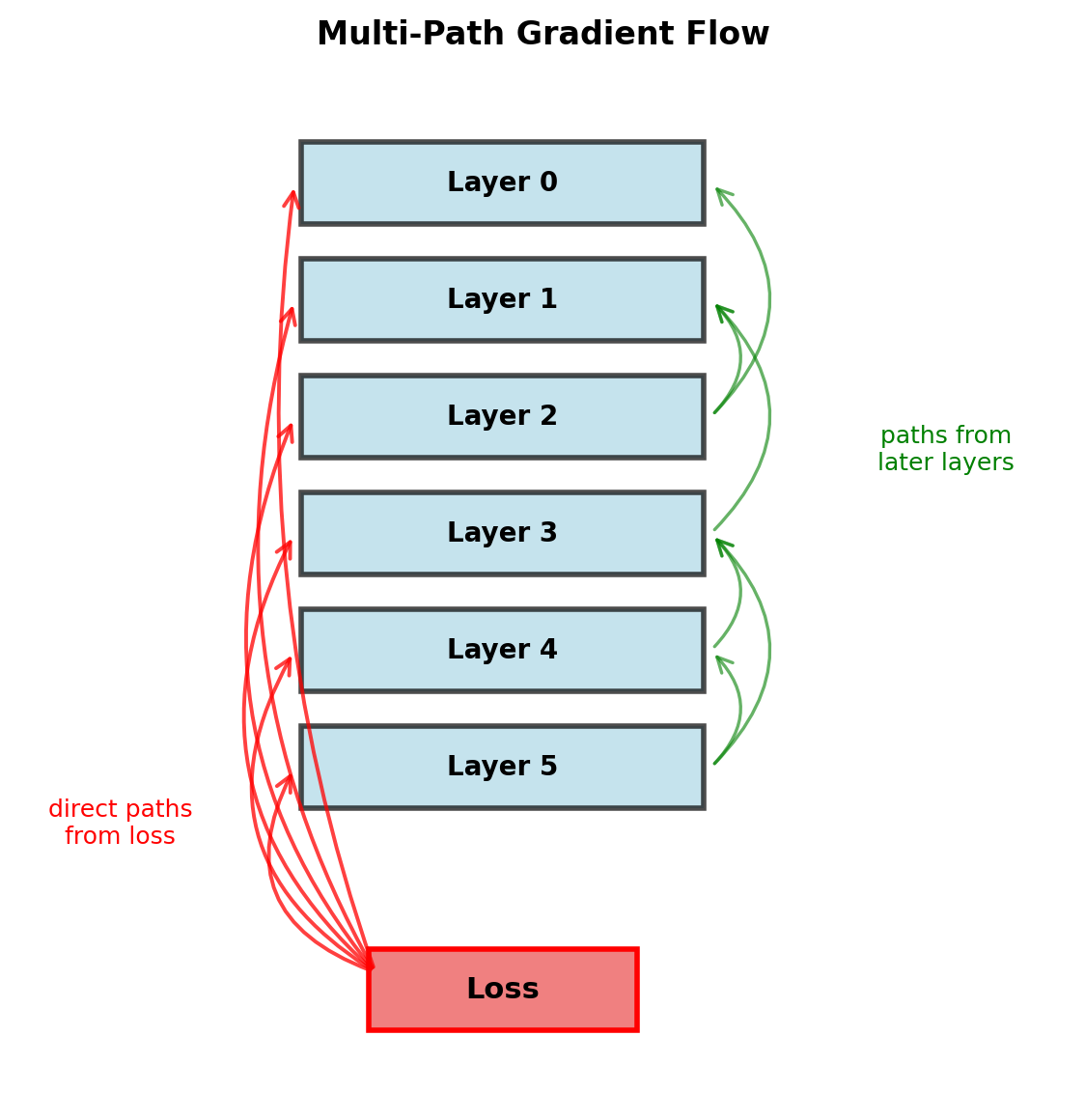
Gradient Flow in DenseNet
Direct Gradient Paths
Loss gradient to layer \(\ell\): \[\frac{\partial \mathcal{L}}{\partial x_\ell} = \frac{\partial \mathcal{L}}{\partial x_L} \frac{\partial x_L}{\partial x_\ell} + \sum_{s=\ell+1}^{L-1} \frac{\partial \mathcal{L}}{\partial H_s} \frac{\partial H_s}{\partial x_\ell}\]
Each layer receives:
- Direct supervision from loss
- Gradient from all subsequent layers
- No transformation through intermediate layers
Implicit Deep Supervision
Shorter paths to loss function → stronger gradient signal
Average path length: \(\frac{L+1}{2}\) (vs \(L\) in sequential)
The Regularization Effect
Dense connections act as implicit regularization:
- Each layer must work with all previous features
- Forces feature complementarity
- Reduces co-adaptation
Feature Reuse Analysis
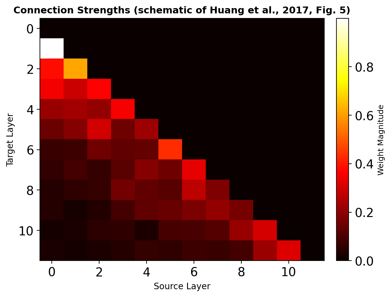
Later layers actively use features from all depths, not just immediate predecessors
Where DenseNet Saves Its Parameters
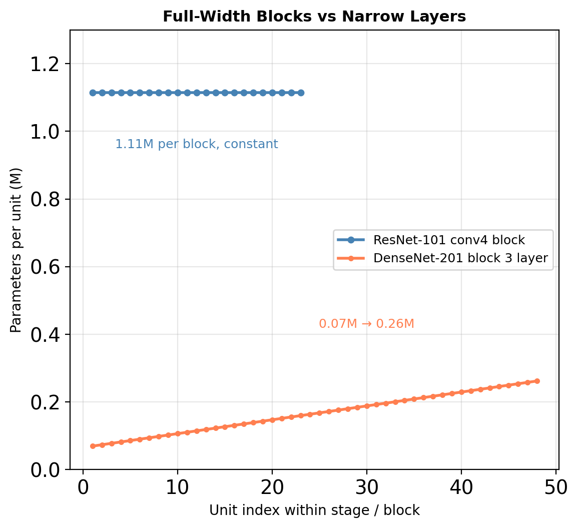
Where Parameters Are Saved
ResNet-101 (44.5M params):
- 33 residual blocks × 3 conv layers
- Each: full channel-to-channel mapping
- Example block: 256→256→1024 channels
DenseNet-201 (20M params):
- Feature reuse via concatenation
- Narrow layers (k=32 new channels)
- Bottleneck: 4k intermediate only
A ResNet block pays for a full-width mapping at every layer. A dense layer pays for one narrow bottleneck — its cost grows only through the 1×1’s input term.
Fewer FLOPs, Harder to Schedule
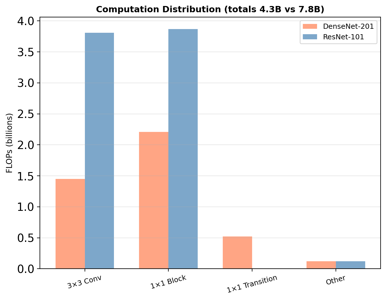
FLOPs Analysis
DenseNet-201: 4.3B FLOPs ResNet-101: 7.8B FLOPs
Despite more connections, fewer FLOPs due to:
- Narrow layers (k=32)
- Efficient bottleneck structure
- Feature reuse
Implementation Challenges
Concatenation overhead:
- Memory allocation
- Data movement
- Cache inefficiency
GPU utilization:
- Many small operations
- Limited parallelism within layers
- Memory bandwidth bound
Successors Prune the O(L²) Connectivity
CondenseNet (2018)
- Learned group convolutions
- Prune connections during training
- 10× fewer FLOPs at same accuracy
SparseNet (2018)
- Exponentially spaced connections
- Connect layer \(i\) to \(i-2^k\) for all valid \(k\)
- \(O(L \log L)\) connections vs \(O(L^2)\)
VoVNet (2019)
- One-shot aggregation
- Aggregate once at block end
- Better GPU utilization
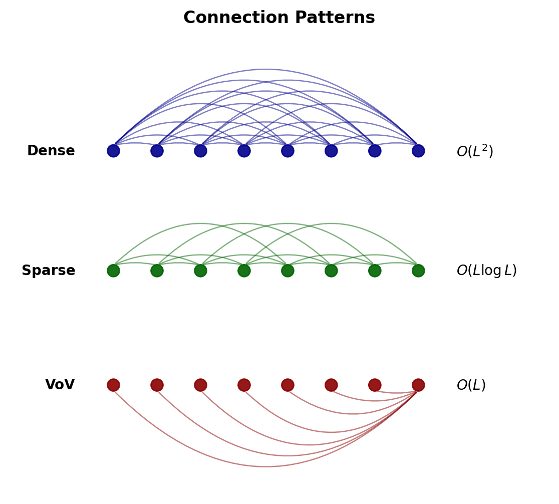
Dense connectivity principle spawned multiple architectural innovations
One Layer Can Exceed the Mobile MAC Budget
Counting unit — the MAC: \(\text{acc} \mathrel{+}= a \cdot b\)
- The multiply–accumulate inside every FIR filter sum
- Convolutions and matmuls decompose into MACs exactly
- Silicon fuses the pair into one unit — a multiplier feeding an adder — replicated by the thousands
- FLOPs counts the two halves separately: 2 FLOPs per MAC
Standard convolution complexity: \[O(K^2 \cdot C_{\text{in}} \cdot C_{\text{out}} \cdot H_{\text{out}} \cdot W_{\text{out}})\]
Example: Single ResNet-50 layer
- Input: 56×56×256
- 3×3 conv → 56×56×256
- Operations: 1.85 × 10⁹ MACs
- Parameters: 590K
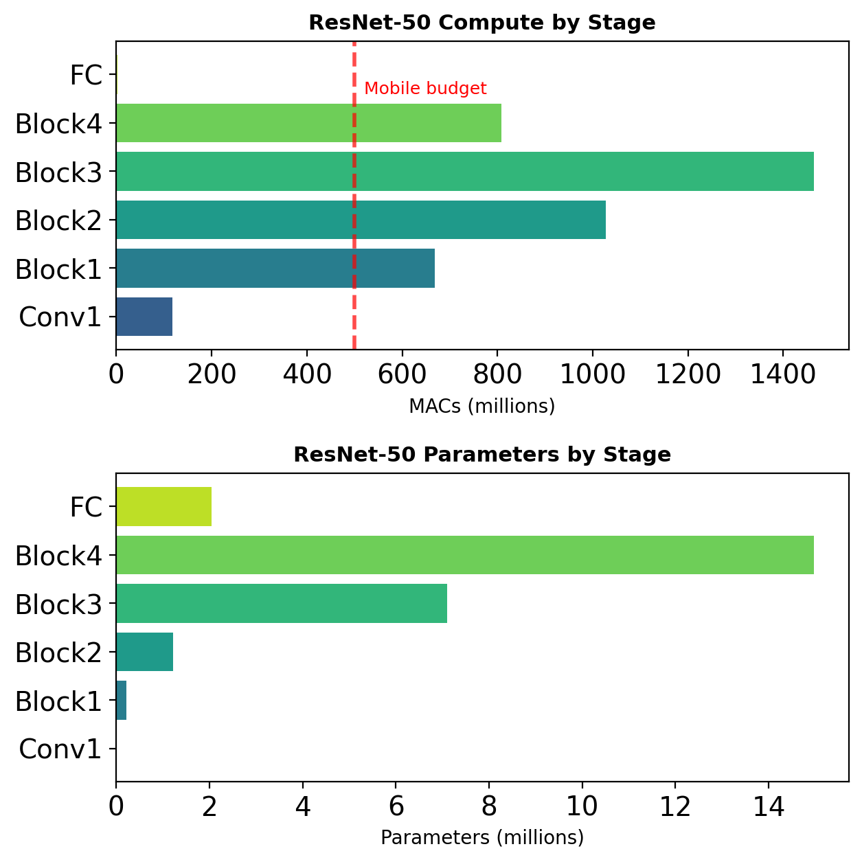
Mobile constraint: <500M MACs total
Convolution Couples Spatial and Channel Mixing
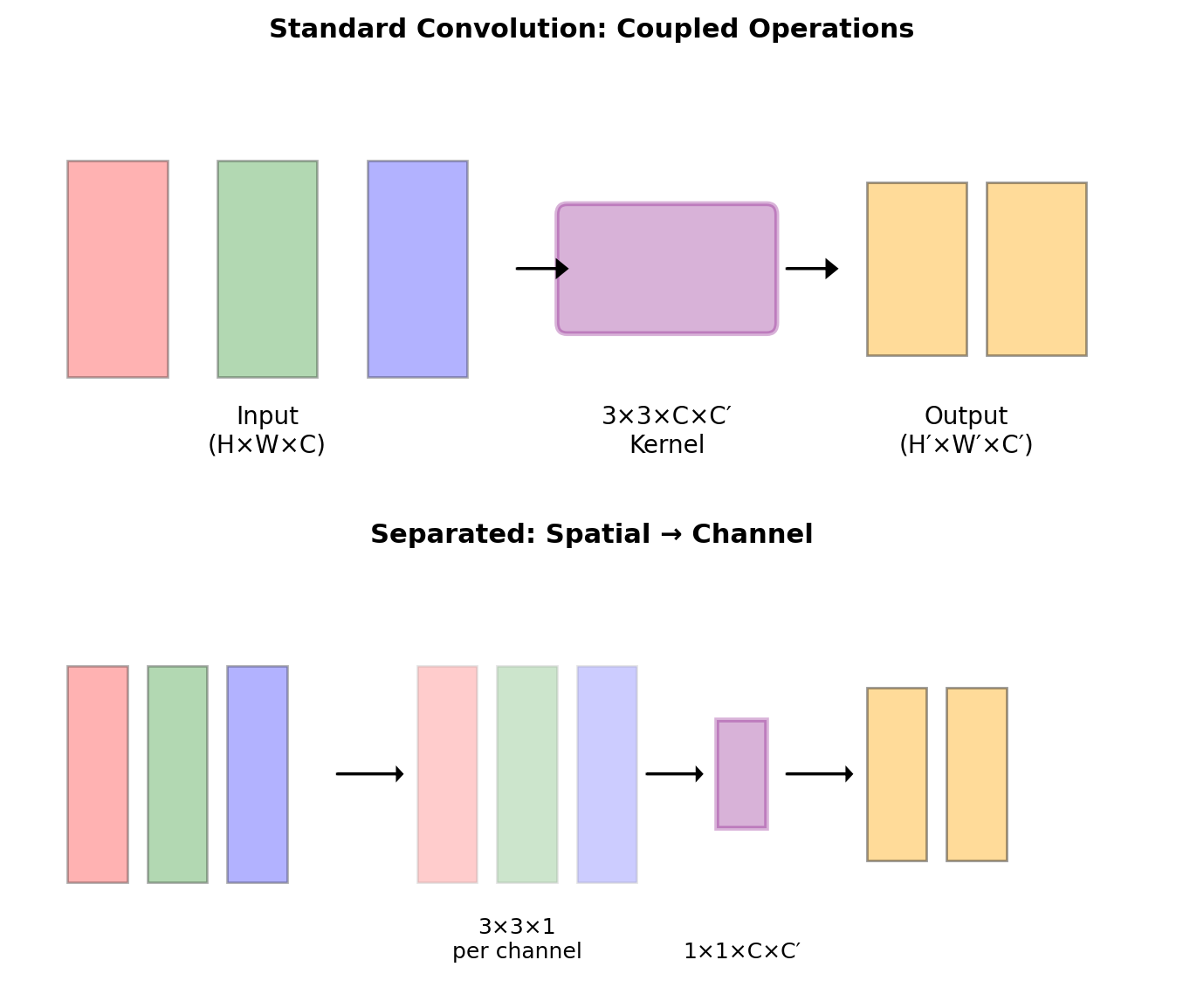
Standard convolution combines two operations:
- Spatial filtering: Aggregate spatial neighbors
- Channel projection: Combine channel information
\[y[i,j,c_o] = \sum_{c_i} \sum_{m,n} h[m,n,c_i,c_o] \cdot x[i+m,j+n,c_i]\]
These operations can be separated for efficiency.
\[y[i,j,c_o] = \sum_{c_i} w[c_i,c_o] \cdot \left(\sum_{m,n} h'[m,n,c_i] \cdot x[i+m,j+n,c_i]\right)\]
Depthwise Convolution: Spatial Filtering Only
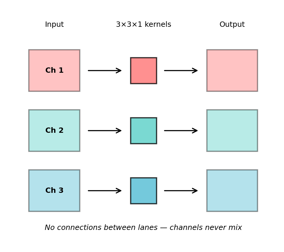
Each input channel convolved with its own \(K \times K\) kernel:
\[\hat{x}[i,j,c] = \sum_{m,n} h_{\text{dw}}[m,n,c] \cdot x[i+m,j+n,c]\]
- No cross-channel mixing
- Channel count unchanged: \(C_{\text{in}} \rightarrow C_{\text{in}}\)
Parameters: \(K^2 \cdot C_{\text{in}}\) (vs \(K^2 \cdot C_{\text{in}} \cdot C_{\text{out}}\) standard)
Example: 3×3 kernel, 16 channels
- Standard: 3×3×16×16 = 2,304 params
- Depthwise: 3×3×16 = 144 params
- 16× reduction
Pointwise Convolution: Channel Mixing Only
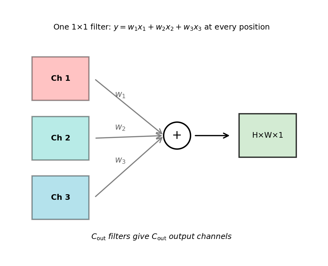
1×1 convolution: linear combination across channels at each position:
\[y[i,j,c_o] = \sum_{c_i} h_{\text{pw}}[c_i,c_o] \cdot \hat{x}[i,j,c_i]\]
- Cross-channel information flow
- No spatial context (1×1 window)
- Spatial resolution preserved
Parameters: \(C_{\text{in}} \cdot C_{\text{out}}\)
Use cases:
- Dimension reduction/expansion
- Bottleneck layers
- Channel mixing after depthwise stage
Example: 256 → 64 channels costs 256×64 = 16,384 params
Depthwise Separable Convolution
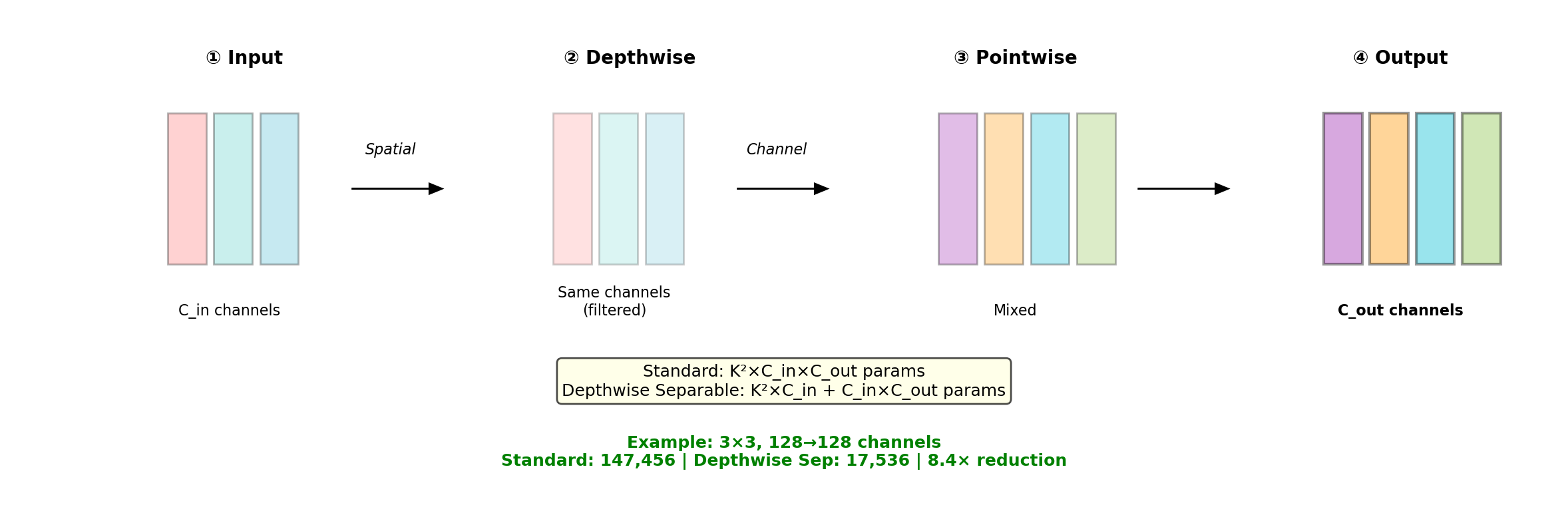
Reduction factor: \[\frac{\text{Depthwise Separable}}{\text{Standard}} = \frac{K^2 C_{\text{in}} + C_{\text{in}} C_{\text{out}}}{K^2 C_{\text{in}} C_{\text{out}}} = \frac{1}{C_{\text{out}}} + \frac{1}{K^2}\]
For \(K=3\): approaches 9× as \(C_{\text{out}}\) grows. At 32→64 channels: 18,432 → 2,336 params (7.9×).
MobileNet V1: 27× Fewer MACs than VGG-16
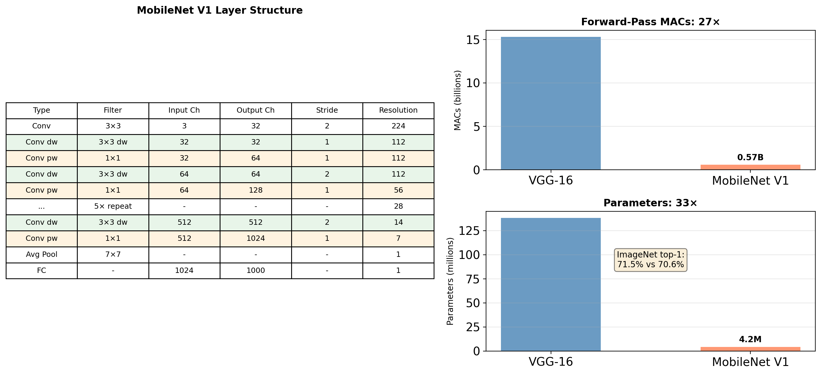
Total: 569M MACs, 4.2M parameters (vs VGG16: 15.3B MACs, 138M parameters)
Width multiplier \(\alpha \in \{1, 0.75, 0.5, 0.25\}\) and input resolution \(\rho \in \{224, 192, 160, 128\}\) scale the family down from there.
MobileNet V2: Expand, Filter, Project Linearly
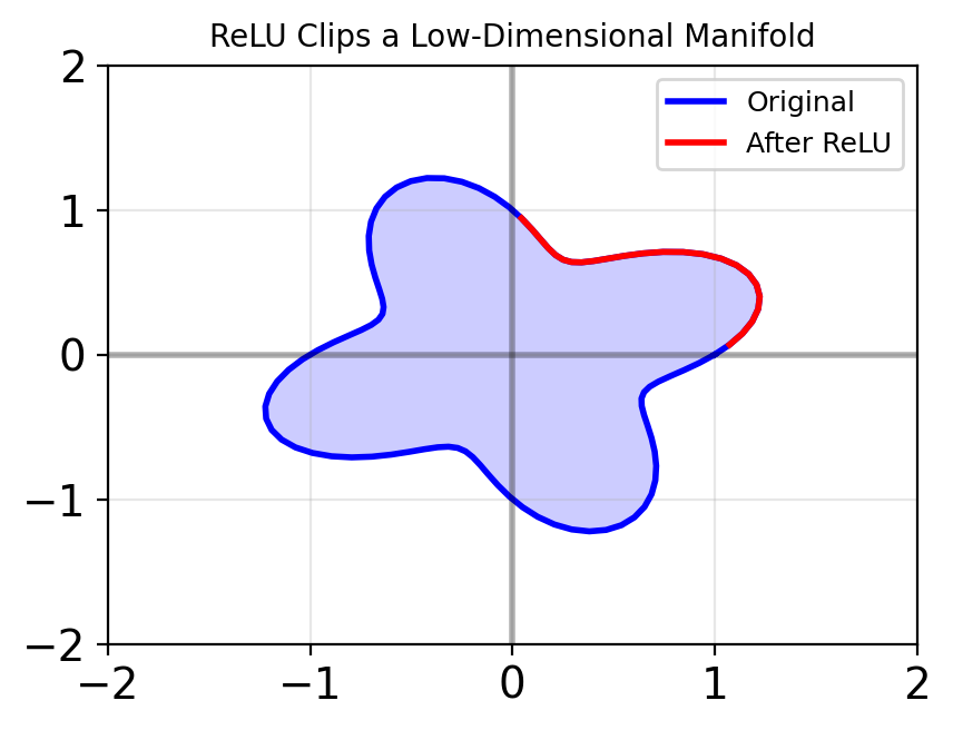
ReLU-induced Collapse
Low-dimensional ReLU causes information loss:
Solution
Linear bottleneck: no activation after projection
Inverted Residual Block
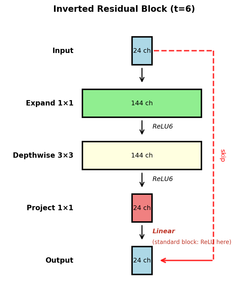
Expansion factor \(t=6\) typical
\(\text{ReLU6}(x) = \min(\max(0, x), 6)\) — the clip bounds the activation range for fixed-point arithmetic
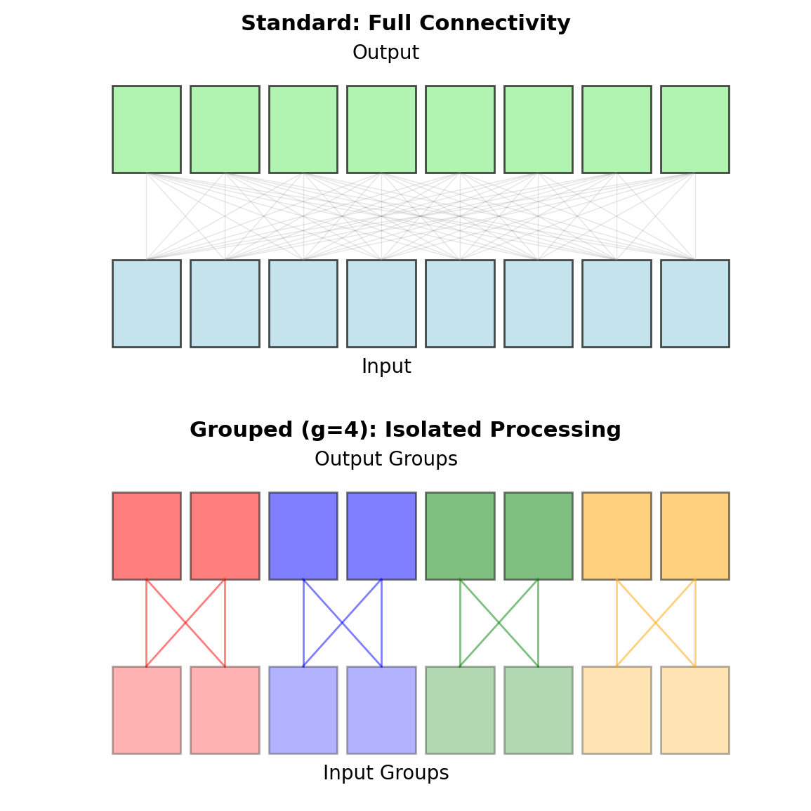
Grouped Convolution: Independent Channel Groups
Divide channels into \(g\) groups, each processed independently:
\[y[i,j,c_o] = \sum_{c_i \in \mathcal{G}(c_o)} \sum_{m,n} h[m,n,c_i,c_o] \cdot x[i+m,j+n,c_i]\]
where \(\mathcal{G}(c_o)\) is the input group for output \(c_o\).
- Originated in AlexNet (splitting across two GPUs)
- Parallelizable: groups have no data dependencies
- Depthwise convolution is the limit case \(g = C_{\text{in}}\)
- Cost: no cross-group information flow
Reduction factor = \(g\) (here: 8×)
Shuffling Restores Cross-Group Flow
The Problem
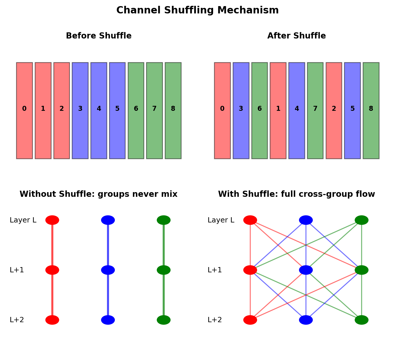
No cross-group information flow → limited representation
The Solution
Deterministic channel permutation:
- Reshape: \((g, n) \rightarrow (g, n)\)
- Transpose: \((g, n) \rightarrow (n, g)\)
- Flatten: \((n, g) \rightarrow (g \cdot n)\)
ShuffleNet: MobileNet Accuracy at Half the MACs
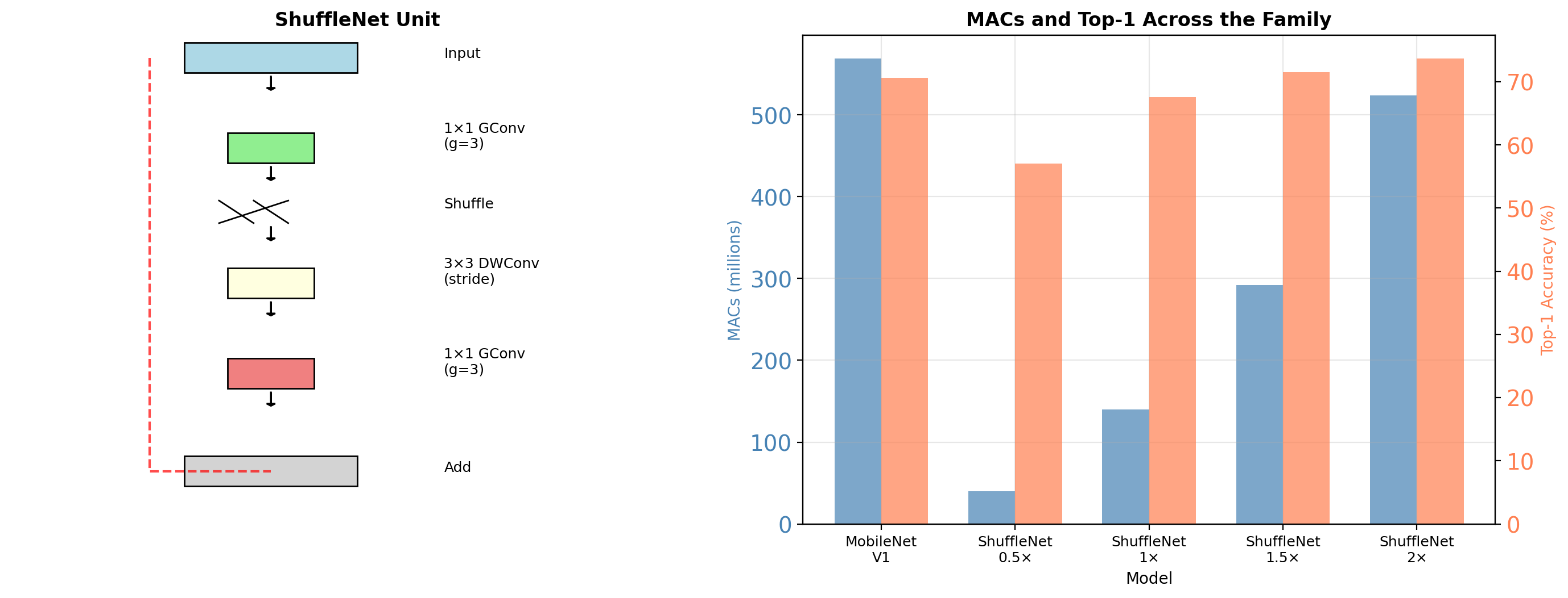
ShuffleNet 1.5× matches MobileNet accuracy with 2× fewer operations
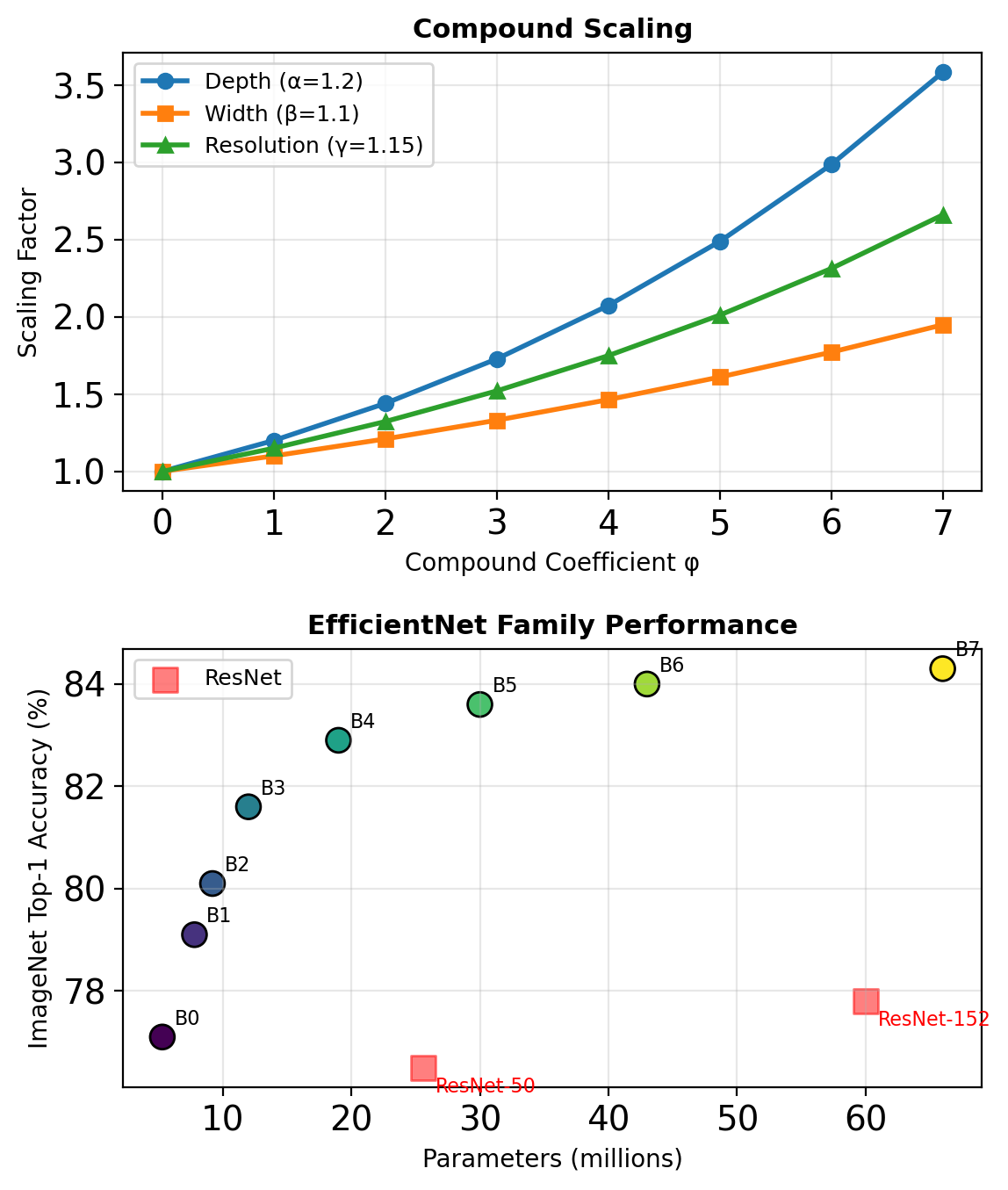
EfficientNet Scales Depth, Width, and Resolution Together
Scaling Dimensions
- Width (w): number of channels
- Depth (d): number of layers
- Resolution (r): input image size
Compound Scaling Rule
Given compound coefficient \(\phi\):
\[\begin{align} \text{depth}: \quad d &= \alpha^\phi \\ \text{width}: \quad w &= \beta^\phi \\ \text{resolution}: \quad r &= \gamma^\phi \end{align}\]
Constraint: \(\alpha \cdot \beta^2 \cdot \gamma^2 \approx 2\)
(FLOPS \(\propto\) width² × resolution²)
For EfficientNet: \(\alpha = 1.2\), \(\beta = 1.1\), \(\gamma = 1.15\)
MobileNetV3: Search Optimized Measured Latency, Not FLOPs
MobileNetV3: Platform-Specific Optimization
Discovered through hardware-aware NAS:
- Redesigned expensive layers
- SE blocks where beneficial
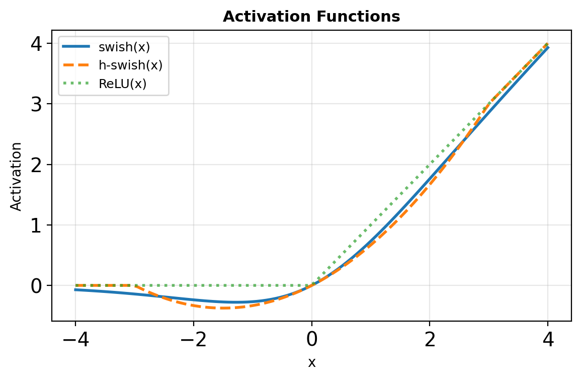
- Hard-swish activation
\[h\text{-}swish(x) = x \cdot \frac{\text{ReLU6}(x+3)}{6}\]
Approximates swish but cheaper:
- No exponential operations
- Bounded output range
- Piecewise linear
Architecture Search Space Evolution
Search pipeline: platform-aware NAS (MnasNet) for the block structure, NetAdapt for per-layer widths, manual redesign of the expensive stem and head.
| MobileNetV2 | MobileNetV3-Large | |
|---|---|---|
| Design | Manual | NAS + manual |
| Parameters | 3.4M | 5.4M |
| ImageNet top-1 | 72.0% | 75.2% |
| Pixel-1 latency | baseline | −20% |
+3.2% accuracy at lower measured latency — the search optimizes phone latency directly, not FLOPs.
Latest Architectures
ConvNeXt (2022): “Modernized” ResNet with depthwise conv, larger kernels (7×7), and transformer-inspired designs. Achieves 87.8% ImageNet with standard convolutions.
EfficientNetV2 (2021): Progressive training with Fused-MBConv blocks. Trains 5-11× faster than V1.
FLOPs ≠ Latency
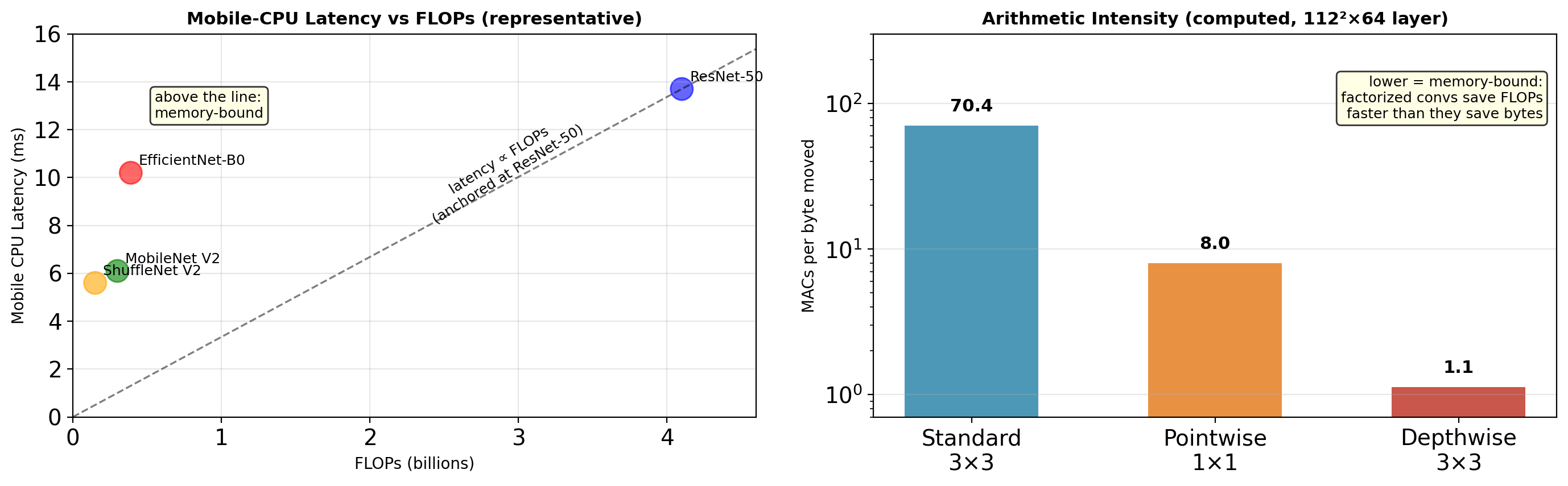
Memory bandwidth often dominates latency on edge devices, not arithmetic operations
Every Layer Has Two Costs: MACs and Bytes
A layer has two costs:
- MACs — arithmetic performed
- Bytes — weights and activations moved through the memory system
The architectures so far reduce MACs:
- Depthwise separable: 8–9× fewer MACs
- Bottlenecks and grouped convolutions: the same term
But measured latency and energy fall by much less — FLOPs ≠ latency.
Arithmetic intensity relates the two:
\[I = \frac{\text{MACs performed}}{\text{bytes moved}}\]
A property of the layer, independent of hardware. Computed for one 112²×64 layer:
- Standard 3×3: \(I = 70.4\) MACs/byte
- Depthwise 3×3: \(I = 1.1\) MACs/byte
Reducing MACs without reducing bytes lowers \(I\): the arithmetic decreases, the memory traffic does not.
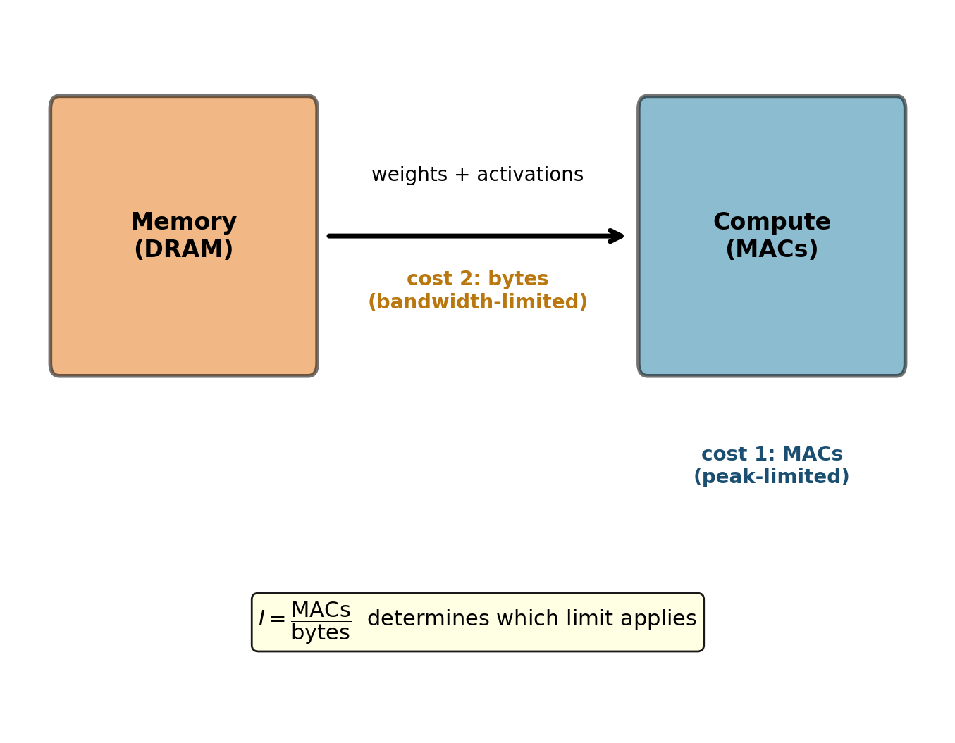
Architecture reduces MACs. Numeric precision reduces bytes.
The Roofline Model Separates Compute-Bound from Memory-Bound
Attainable throughput is the minimum of two limits:
\[\text{MACs/s} = \min\left(\text{peak}, \; \text{bandwidth} \times \frac{\text{MACs}}{\text{byte}}\right)\]
Machine balance — the crossover intensity:
\[\frac{\text{peak}}{\text{bandwidth}} = \frac{9{,}750 \text{ GMAC/s}}{1{,}555 \text{ GB/s}} \approx 6.3 \; \text{MACs/byte}\]
(A100, FP32)
Below balance, the arithmetic units wait on memory. A higher peak rate does not help.
The three convolution types at their computed intensities:
- Standard 3×3: 70.4 MACs/byte — compute-bound
- Pointwise 1×1: 8.0 — near balance
- Depthwise 3×3: 1.1 — memory-bound, runs at ~18% of peak
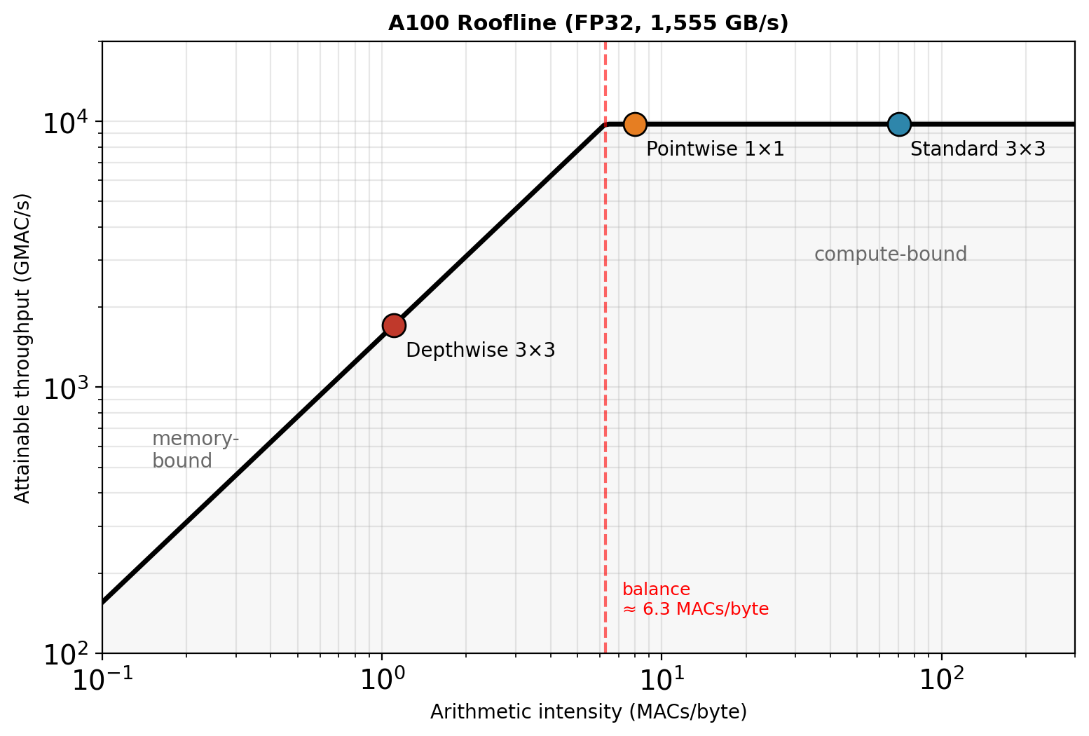
Architecture design reduces FLOPs. Below the balance point, only reducing bytes helps.
Inference Cost Is Counted in Bytes
Every forward pass moves two kinds of bytes:
| FP32 | ResNet-50 | MobileNetV2 |
|---|---|---|
| Weights | 102 MB | 14 MB |
| Peak activation (batch 1) | 3.2 MB | 4.6 MB |
| Weight traffic per image (batch 1) | 102 MB | 14 MB |
At batch 1, all weights are read for every image:
\[\frac{102 \text{ MB}}{1{,}555 \text{ GB/s}} \approx 66 \; \mu\text{s}\]
— a lower bound on latency before the first MAC executes. Batching amortizes weight reads. Edge inference rarely has a batch.
Moving bytes also dominates energy (45 nm, Horowitz 2014):
- FP32 multiply: 3.7 pJ
- 32-bit read from DRAM (off-chip memory): 640 pJ — 170× the multiply
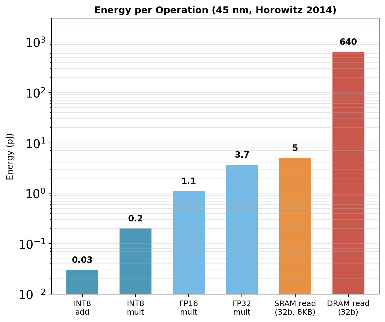
Bytes per value is the one parameter that scales weights, activations, bandwidth, and energy together.
FP32 Anatomy: Sign, Exponent, Mantissa
Reducing bytes per value means changing the number format. The starting point is what FP32’s 32 bits encode.
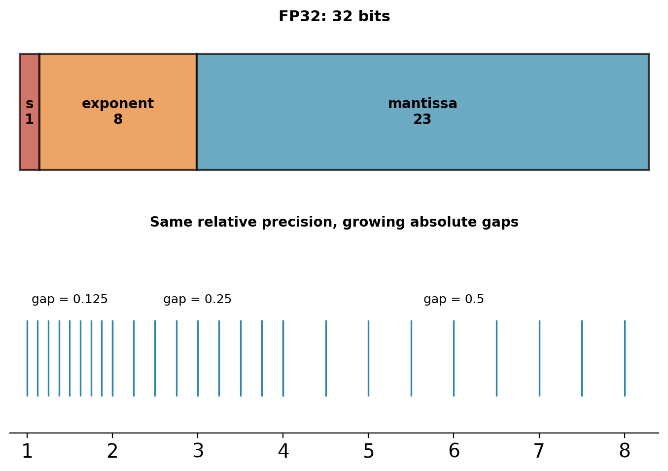
\[v = (-1)^s \times 1.m \times 2^{\,e - 127}\]
| Field | Bits | Controls |
|---|---|---|
| Sign \(s\) | 1 | polarity |
| Exponent \(e\) | 8 | dynamic range: ±3.4×10³⁸ |
| Mantissa \(m\) | 23 | relative precision: \(2^{-23} \approx 1.2\times10^{-7}\) |
- Exponent bits determine range: which magnitudes are representable
- Mantissa bits determine precision: the spacing between values, relative to magnitude
Representable values form a geometric grid: the gap between neighbors is proportional to magnitude. Absolute error grows with scale. Relative error stays \(\approx 2^{-(\text{mantissa bits})}\).
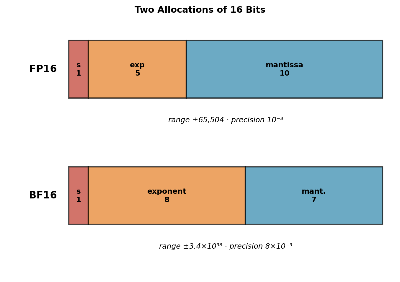
FP16 and BF16 Split the Same 16 Bits Differently
| FP16 | BF16 | |
|---|---|---|
| Layout | 1 / 5 / 10 | 1 / 8 / 7 |
| Max value | 65,504 | ~3.4×10³⁸ |
| Min normal | 6.1×10⁻⁵ | 1.2×10⁻³⁸ |
| Relative precision | \(2^{-10} \approx 10^{-3}\) | \(2^{-7} \approx 8\times10^{-3}\) |
FP16: more precision, less range.
- Gradients routinely fall below \(6\times10^{-5}\) → silent flush to zero
- Requires loss scaling (treated with transformer training)
BF16: FP32’s exponent, less precision.
- Same range as FP32: drop-in replacement, no loss scaling
- 3 decimal digits → sufficient for weights and activations, marginal for accumulation
One allocation decision: range vs precision, 16 bits total.
INT8: Integer Arithmetic, Not Just Smaller Floats
Integers have no per-value exponent — a fixed uniform grid:
- 256 levels, \([-128, 127]\)
- One shared scale factor per tensor (or per channel) maps the grid onto the reals
- Constant absolute spacing, so relative precision degrades toward zero
Consequences in silicon:
- Multiplier circuit area grows ~quadratically with operand width: an 8-bit multiplier is a small fraction of an FP32 unit
- No exponent alignment before the add, no renormalization after
- 0.2 pJ vs 3.7 pJ per multiply (18×)
- 4× more values per byte of bandwidth
The cost: one shared scale must represent the whole tensor. Choosing the scale, and measuring the resulting error, is a quantization problem.
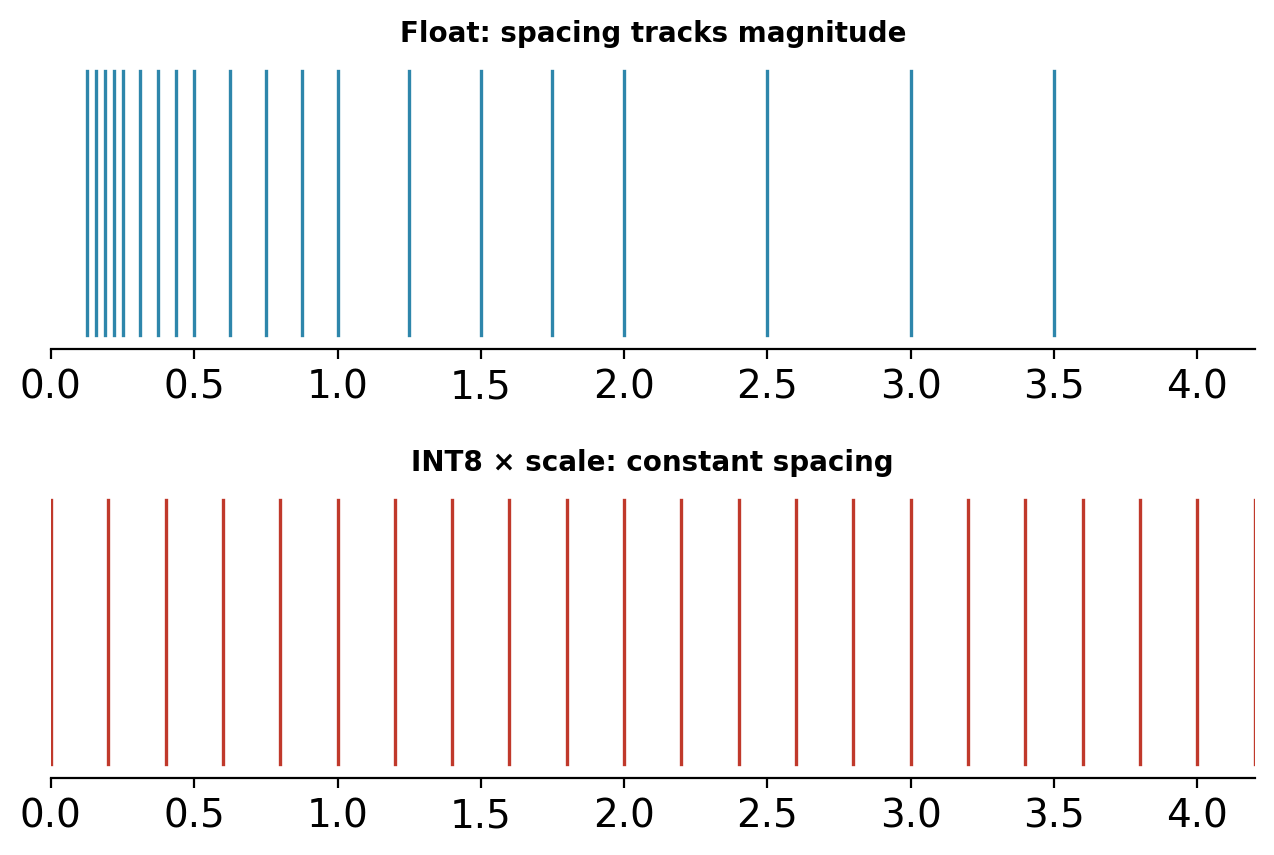
Uniform spacing allows pure integer MACs.
Two FP8 Formats: E4M3 for Forward, E5M2 for Gradients
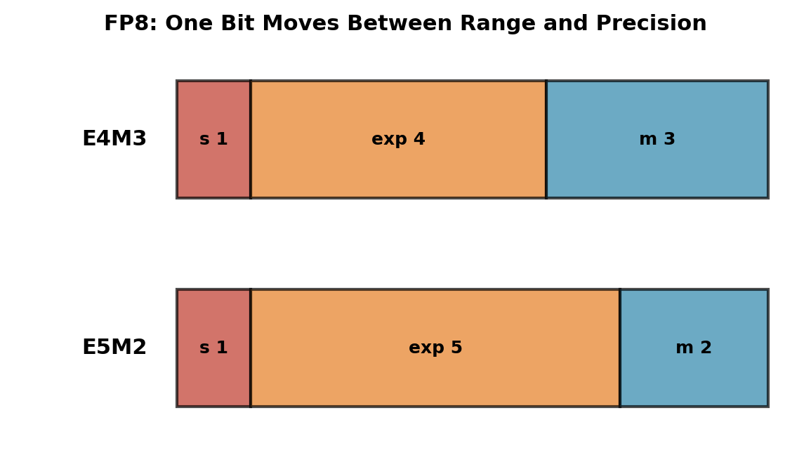
Two standardized 8-bit floats. The name gives the field widths (E4M3: 4 exponent bits, 3 mantissa bits):
| E4M3 | E5M2 | |
|---|---|---|
| Layout | 1 / 4 / 3 | 1 / 5 / 2 |
| Max | 448 | 57,344 |
| Relative precision | ~6% | ~12% |
| Used for | weights, activations | gradients |
The same range-vs-precision allocation at 8 bits:
- Forward tensors are well-scaled → allocate bits to mantissa (E4M3)
- Gradients span many orders of magnitude → allocate bits to exponent (E5M2)
Hardware support arrived with H100 tensor cores (2022). FP8 training runs with FP32 accumulation and per-tensor scaling.
FP8 is used for transformer training and serving. CNN deployment standardized on INT8.
Sub-Byte Formats Pack Multiple Weights per Byte
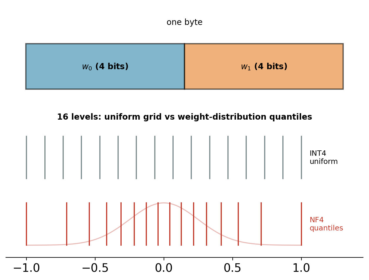
INT4: 16 levels, two weights per byte.
- Too coarse for a whole tensor under one scale
- Group-wise scales: one FP16 scale per 64–128 weights
- Effective cost: ~4.2 bits/weight including scales
NF4: 16 levels placed at the quantiles of a Gaussian — a codebook, not a uniform grid. Matches the distribution of trained weights: levels are dense where the weights are.
Sub-byte quantization is standard for LLMs, not CNNs:
- Autoregressive decoding at batch 1 is weight-memory-bound (the roofline’s far left)
- Halving weight bytes ≈ halving decode latency
- Weight-only: activations stay FP16 — weights are dequantized inside the matmul
- CNNs at INT4 lose measurable accuracy and are rarely this memory-bound
The 4-bit methods — GPTQ, AWQ, QLoRA — are large-language-model techniques.
Throughput Follows the Format
Dense (non-sparsity) tensor-core rates:
| A100 | Peak |
|---|---|
| FP32 | 19.5 TFLOPS |
| TF32 (tensor core) | 156 TFLOPS |
| FP16 / BF16 | 312 TFLOPS |
| INT8 | 624 TOPS |
| H100 | Peak |
|---|---|
| BF16 | 989 TFLOPS |
| FP8 | 1,979 TFLOPS |
TF32: a 19-bit tensor-core-internal format — FP32’s exponent, FP16’s mantissa. TOPS: integer operations per second, the INT counterpart of FLOPS.
Bytes shrink by the same factor: INT8 moves 4× the values per unit bandwidth of FP32.
Which gain applies depends on position on the roofline:
- Compute-bound layers gain from the higher peak
- Memory-bound layers gain from the smaller bytes
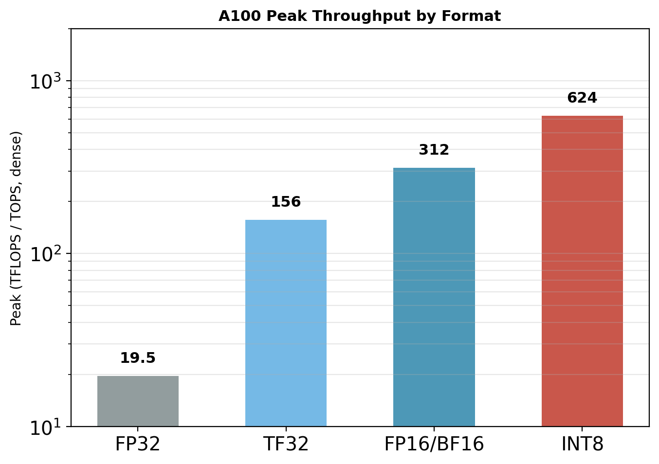
32× from FP32 to INT8, usable only if accuracy holds in the narrower format.
256 Levels Must Cover What Training Produced
An FP32-trained network must run on an integer grid.
Two tensor families, two different problems:
Weights — fixed before deployment.
- Every value inspectable, ranges exact
- Quantization is a one-time compile step
Activations — different for every input.
- Only the distribution is knowable, estimated from sample data
- The grid must be chosen before the inputs arrive
Two questions decide the outcome:
- Where does the grid go? — a range/scale per tensor, an estimation problem
- What does rounding cost? — measured in task accuracy, not MSE
A poor scale collapses accuracy outright. Calibrated per-channel INT8 loses under 0.5%.
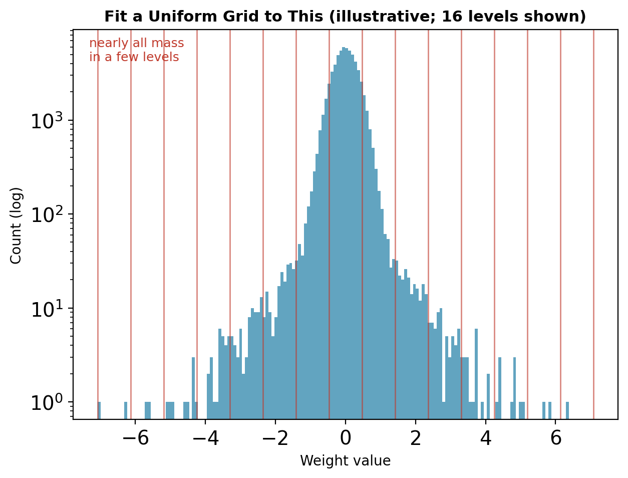
Heavy-tailed values, uniform grid, a fixed number of levels.
Uniform Affine Quantization: A Grid Over the Reals
Map reals to integers with two parameters — a scale \(s\) and a zero-point \(z\):
\[x_q = \text{clip}\!\left(\text{round}\!\left(\frac{x}{s}\right) + z,\; q_{\min},\; q_{\max}\right)\]
Recover an approximation by inverting:
\[\hat{x} = s \,(x_q - z)\]
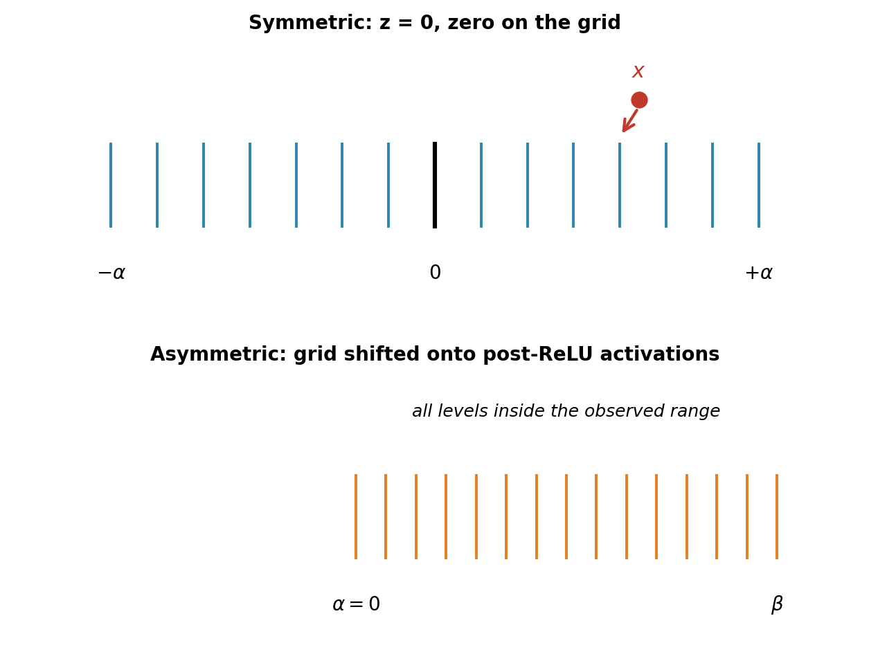
Symmetric (\(z = 0\)): grid centered at zero, \(s = \alpha / 127\) for range \([-\alpha, \alpha]\) in INT8.
- Natural for weights — distributions center on zero
- Zero is represented exactly
Asymmetric: \(s = (\beta - \alpha)/255\), \(z\) shifts the grid.
- Natural for post-ReLU activations — one-sided, \([0, \beta]\)
- Assigns no levels to values that cannot occur
Noise analysis, calibration, and training all concern the choice of \(s\) and \(z\).
Quantization Is Additive Noise: 6 dB per Bit
Model rounding as an additive noise channel:
\[\hat{x} = x + e, \qquad e \sim \text{Uniform}\left(-\tfrac{\Delta}{2}, \tfrac{\Delta}{2}\right)\]
Noise power:
\[\sigma_e^2 = \frac{1}{\Delta}\int_{-\Delta/2}^{\Delta/2} e^2 \, de = \frac{\Delta^2}{12}\]
For \(b\) bits spanning \([-\alpha, \alpha]\): \(\Delta = 2\alpha/2^b\), so
\[\sigma_e^2 = \frac{\alpha^2}{3} \cdot 2^{-2b}\]
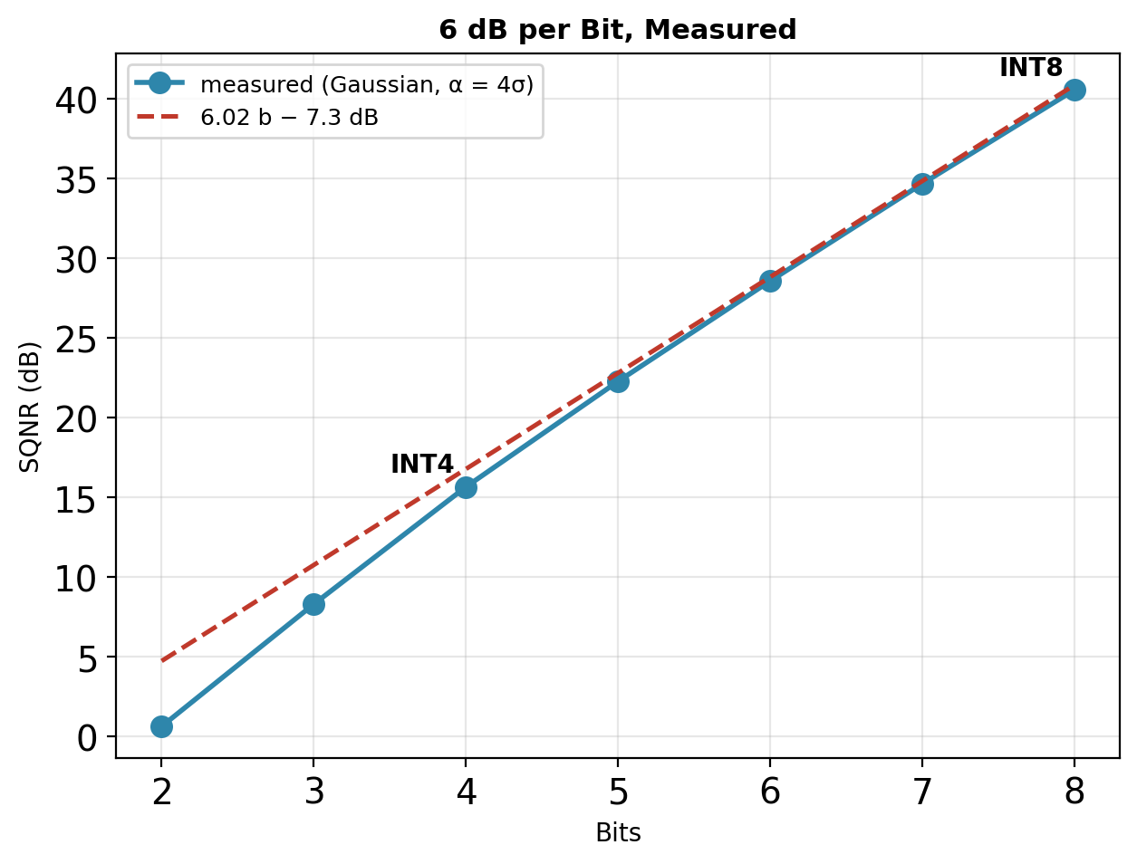
\[\text{SQNR} = 10\log_{10}\frac{\sigma_x^2}{\sigma_e^2} \approx 6.02\,b + \text{const dB}\]
Each bit adds 6 dB. The constant is set by the loading factor \(\alpha/\sigma_x\) — how much headroom the range leaves. At 4σ loading:
- INT8: ~41 dB — quantization noise far below the noise floor SGD already tolerates
- INT4: ~16 dB — noise becomes visible in the task loss
The quantizer is a channel. Bit width sets its SNR.
Assumes fine spacing and no clipping. Choosing \(\alpha\) deliberately violates the second assumption.
Optimal Quantization Ranges Clip Outliers
Two error sources move in opposite directions as the clip threshold \(\alpha\) grows:
- Granular noise \(\propto \Delta^2 \propto \alpha^2\) — a wider range coarsens the grid everywhere
- Clipping distortion — mass beyond \(\pm\alpha\) is pinned to the boundary, shrinking as \(\alpha\) grows
\[\text{MSE}(\alpha) = \underbrace{\frac{(2\alpha/2^b)^2}{12}\,P(|x| \le \alpha)}_{\text{granular}} + \underbrace{\mathbb{E}\big[(|x| - \alpha)^2 \,;\, |x| > \alpha\big]}_{\text{clipping}}\]
Trained weights are heavy-tailed. Min/max range — \(\alpha = \max|x|\) — gives exact representation of a few outliers and coarse resolution for the entire body.
The optimum clips. For a Laplacian tensor at 4 bits, the best \(\alpha\) clips the top fraction of a percent of the mass and reduces total error ~5× vs min/max.
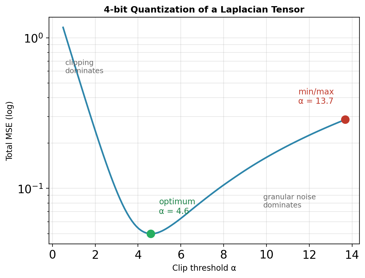
Range selection is a granular-vs-clipping optimization. Calibration methods approximate this optimum from data.
Per-Channel Scales Allocate Resolution Where It’s Needed
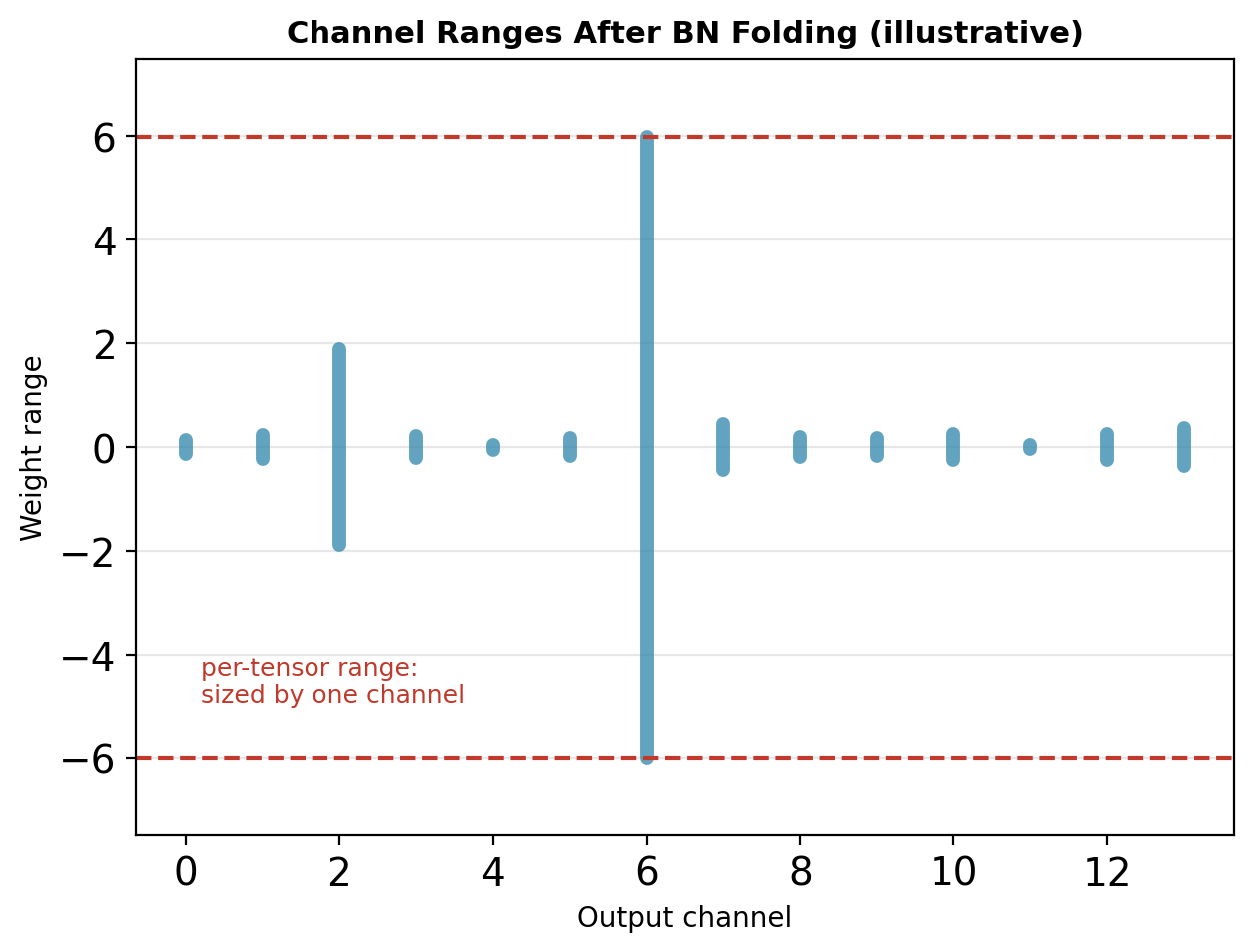
One scale per tensor forces every output channel onto the same grid — and channel weight ranges routinely differ by 10–100×:
- Filters learn at different magnitudes
- BN folding multiplies each channel by its own \(\gamma_c / \sigma_c\), amplifying the spread
- Depthwise layers: 9 weights per channel — extreme ranges are not averaged away
Per-channel quantization: one scale \(s_c\) per output channel, weights only.
\[\hat{W}[c, :] = s_c \, W_q[c, :]\]
Free at inference — \(s_c\) factors out of each output row of the matmul. Activations stay per-tensor.
Measured consequence (Nagel et al., 2019, ImageNet top-1):
| MobileNetV2, W8A8 PTQ | Top-1 |
|---|---|
| FP32 | 71.7% |
| Per-tensor | 0.1% |
| Per-channel | 71.2% |
One scale per channel is the difference between broken and working.
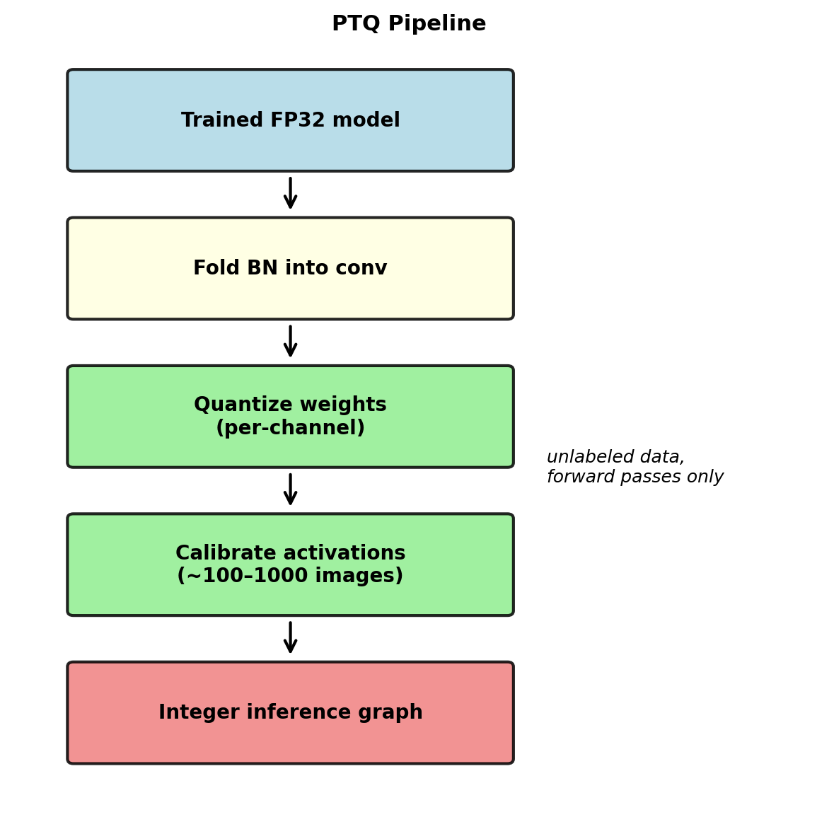
Post-Training Quantization: Calibrate, Don’t Retrain
No labels, no gradients, minutes of work:
- Fold BatchNorm into the preceding convolution: \[W' = \frac{\gamma}{\sigma}\,W \qquad b' = \frac{\gamma\,(b - \mu)}{\sigma} + \beta\]
- Quantize weights — per-channel, directly from the tensors
- Calibrate activations — run ~100–1000 unlabeled images, record ranges per layer
- Fix activation scales, export the integer graph
The only estimation problem is step 3 — activation ranges depend on data:
- Min/max: exact range of the calibration set, so one outlier activation sets the scale
- Percentile (99.9–99.999): clip the tail deliberately
- Entropy / KL (TensorRT): choose \(\alpha\) minimizing information lost between the FP32 and quantized distributions
All three are approximations of the clipping-trade optimum, estimated from a few hundred images.
Quantization-Aware Training: Fake Quantization in the Forward Pass
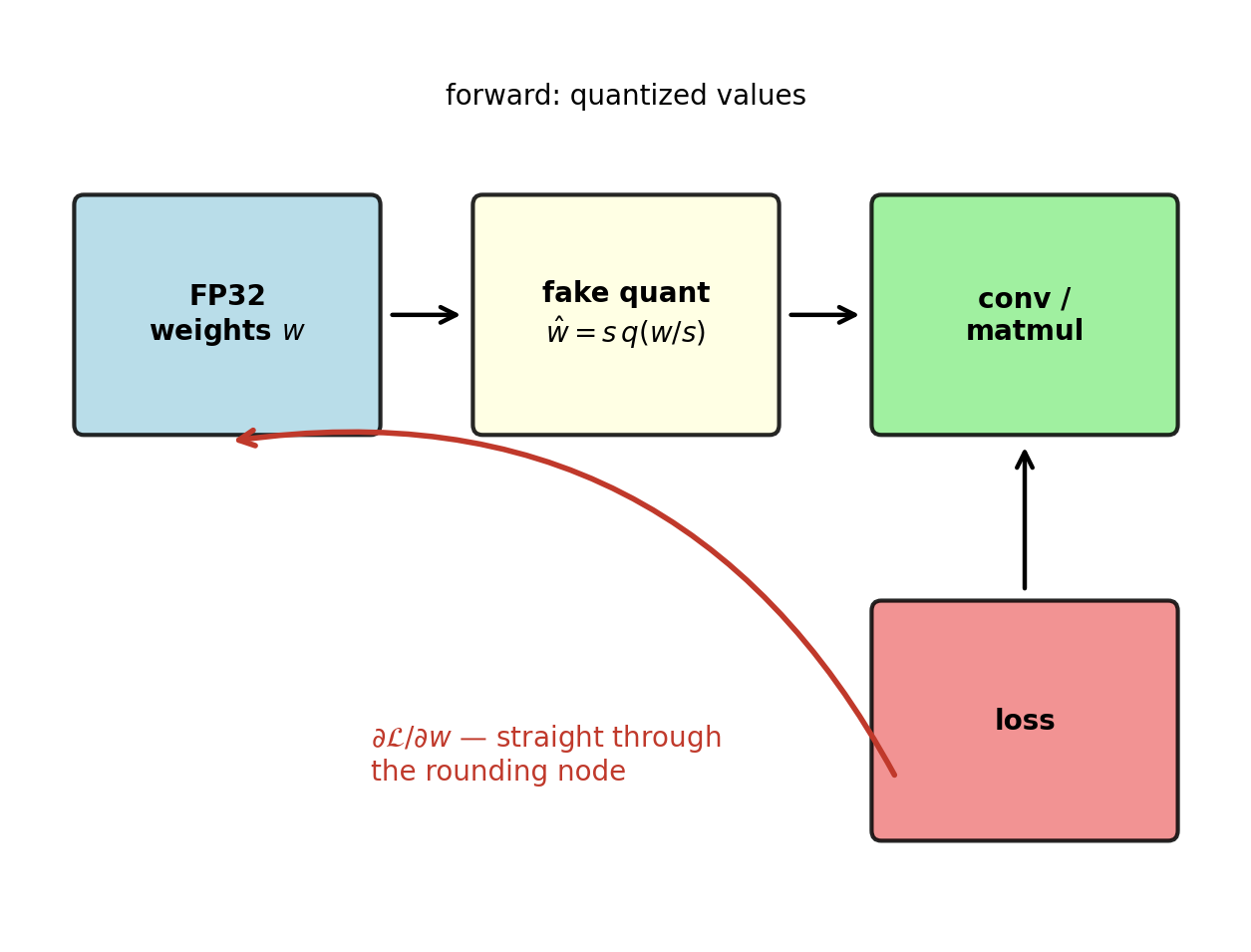
Insert quantize→dequantize nodes into the training graph:
\[w \;\rightarrow\; \underbrace{s\,\text{clip}\!\left(\text{round}(w/s)\right)}_{\text{fake quant}} \;\rightarrow\; \text{conv} \;\rightarrow\; \ldots\]
- Forward: the network computes with quantized values — the loss sees exactly the deployed arithmetic
- Backward: gradients update the FP32 shadow weights. The integer grid is only a view
- Applied to weights and activations, with scales fixed from calibration or learned as parameters (LSQ)
Training adapts to the grid:
- Weights move toward representable points
- Training finds minima less sensitive to quantization
- Scales converge to the granular-vs-clipping optimum for the task loss, not for MSE
One obstacle: the round function has no useful gradient.
The Straight-Through Estimator
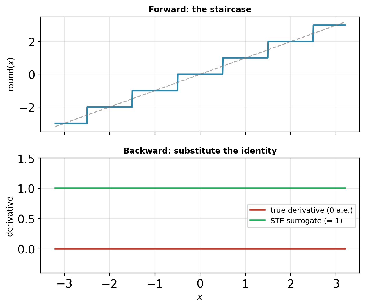
Rounding is a staircase:
\[\frac{\partial\, \text{round}(x)}{\partial x} = 0 \quad \text{almost everywhere}\]
Backpropagated exactly, every weight gradient is zero at the fake-quant node.
STE: replace the true derivative with the identity inside the representable range:
\[\frac{\partial \hat{w}}{\partial w} := \begin{cases} 1 & |w| \le \alpha \\ 0 & |w| > \alpha \end{cases}\]
\[\frac{\partial \mathcal{L}}{\partial w} = \frac{\partial \mathcal{L}}{\partial \hat{w}} \cdot \mathbb{1}[|w| \le \alpha]\]
- Forward uses the real staircase. Backward substitutes the identity
- Clipped weights receive zero gradient — outside the representable range, no update
- Biased estimator with no convergence guarantee, reliable empirically
The same surrogate trains VQ-VAE codebooks through their discrete bottleneck: gradients copied straight through the nearest-neighbor lookup.
Trained Networks Are Mostly Redundant
Three ways to compress a network:
- Bits per value — quantization
- Number of values — pruning
- Size of the model — distillation
Evidence that values can go (Han et al., 2015, ImageNet, no accuracy loss):
| Weights | Pruned | Ratio | |
|---|---|---|---|
| AlexNet | 61M | 6.7M | 9× |
| VGG-16 | 138M | 10.3M | 13× |
Where the redundancy is:
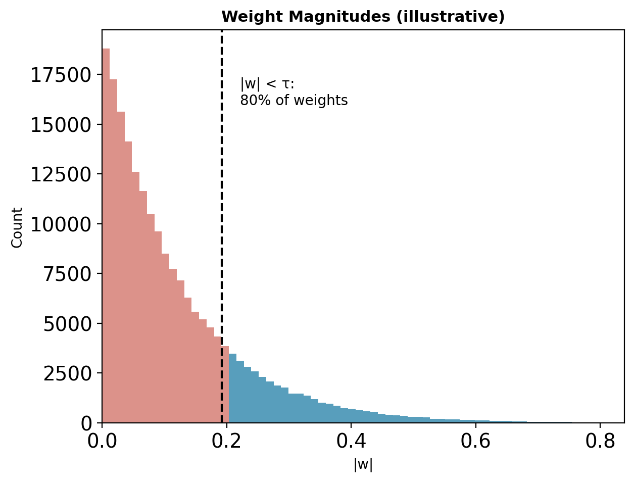
- Trained weight magnitudes concentrate near zero
- FC layers: ~91% removable (AlexNet)
- Conv layers: ~60–70% removable
Over-parameterization aids optimization. Inference does not need it.
Magnitude Pruning: Remove, Fine-Tune, Repeat
Criterion: remove weights with \(|w| < \tau\) — threshold per layer or global.
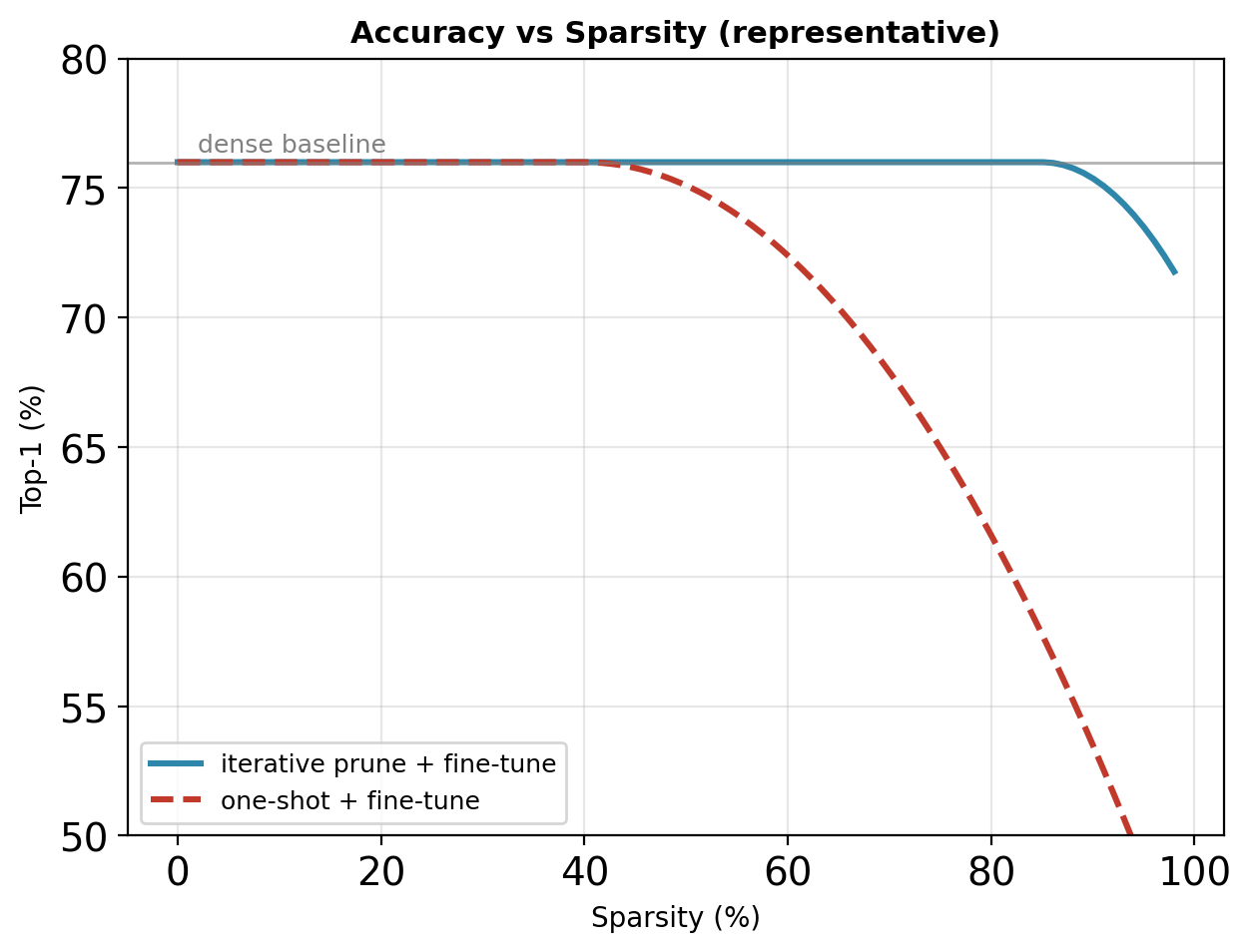
One-shot — prune to target sparsity, fine-tune once:
- Works to moderate sparsity (~50–70%)
- Several % accuracy loss at 90%
Iterative — prune a fraction, fine-tune, repeat:
- Each round, fine-tuning adjusts the remaining weights to compensate
- Reaches 80–90% sparsity at full accuracy (the 9–13× results)
- Cost: multiple fine-tuning cycles
Fine-tuning is not optional — pruning without retraining loses accuracy at any useful sparsity.
Sparse subnetworks at these ratios can be trained from initialization in isolation (Frankle & Carbin, 2019) — the redundancy exists before training, not only after.
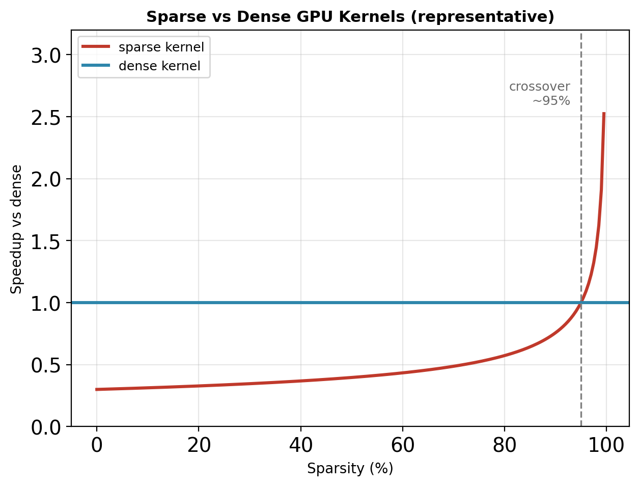
Unstructured Sparsity Does Not Make GPUs Faster
Removed weights leave zeros scattered through the tensor, not a smaller tensor.
Storage: sparse formats keep values plus indices.
- One index per surviving value
- At 50% sparsity with 32-bit indices: larger than the dense tensor
Compute: the MAC array does not skip zeros.
- Dense kernels process the zeros at full cost
- Sparse kernels break coalesced memory access and idle the tensor cores
- Crossover vs dense: ~95%+ sparsity on GPU
What unstructured sparsity delivers:
- Smaller compressed storage and transmission
- Energy savings on hardware with zero-skipping
- Not latency on standard GPU inference
90% of the weights removed, 0% faster: the sparsity pattern does not match what the hardware can use.
Structured Sparsity Trades Granularity for Speed
Constraining where the zeros go restores the hardware speedup.
Channel pruning — remove whole filters:
- The result is a smaller dense network — every dense-kernel and architecture result applies
- A channel-pruned ResNet is a narrower ResNet
- Coarsest granularity: largest accuracy cost per removed weight
2:4 semi-structured (Ampere tensor cores):
- Exactly 2 of every 4 consecutive weights zero
- Tensor cores skip the zero pairs: 2× peak — the sparse column of the spec sheet
- Fine granularity, fixed 50% sparsity, ~0 accuracy loss with fine-tuning
The trade at fixed sparsity:
- Finer granularity → better accuracy, less hardware benefit
- Coarser granularity → real speedup, larger accuracy cost
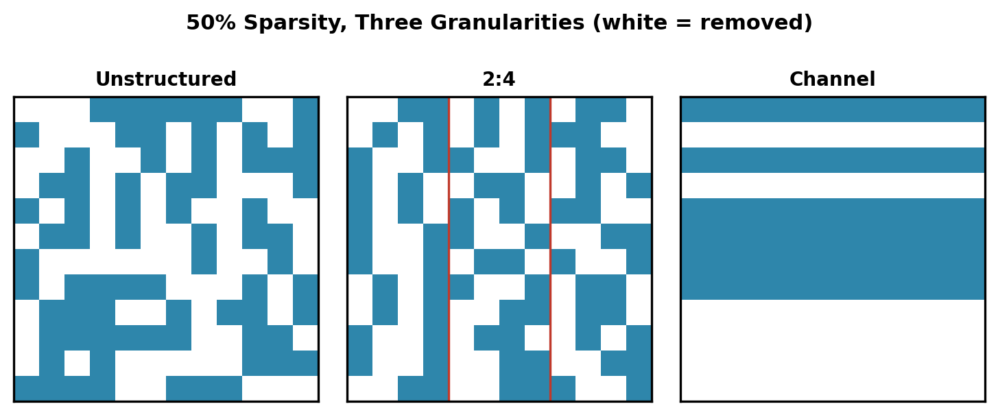
Same fraction removed. Only the two right patterns change what the hardware executes.
Distillation: Train the Student on Soft Targets
A large trained teacher supervises a small student.
Temperature-softened outputs:
\[p_i^{(T)} = \frac{\exp(z_i / T)}{\sum_j \exp(z_j / T)}\]
- \(T = 1\): ordinary softmax
- \(T > 1\): flattened distribution, small logits become visible
- Typical \(T = 2\)–\(5\)
Student loss — hard labels plus teacher match:
\[\mathcal{L} = (1 - \lambda)\, \text{CE}(y, p_S) + \lambda\, T^2\, \text{KL}\!\left(p_T^{(T)} \,\|\, p_S^{(T)}\right)\]
- The \(T^2\) factor keeps the soft-target gradients at the same magnitude as the hard-label gradients
- The KL term is the soft-label cross-entropy from the loss-function review, with the teacher supplying the labels
The teacher runs once per example. Only the student trains.
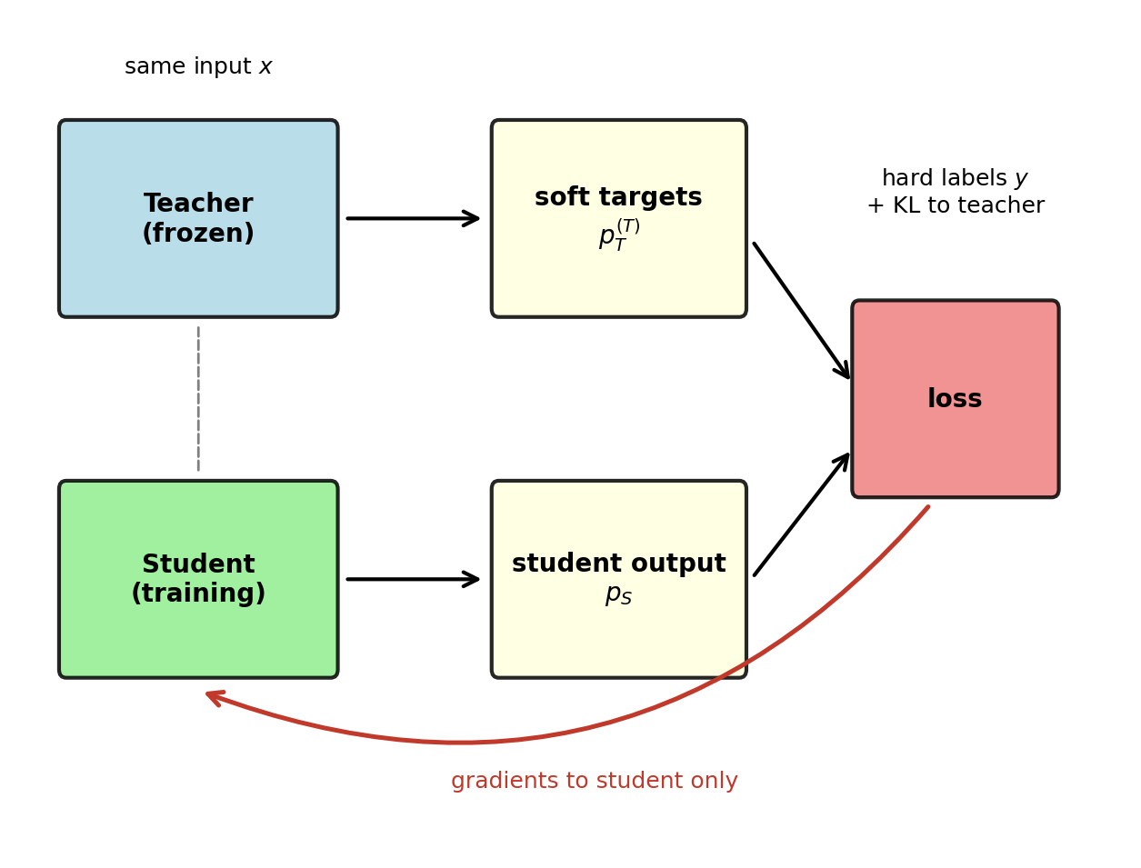
Dark Knowledge: Wrong Answers Carry Information
A hard label carries the class. The teacher’s full distribution carries the class and its similarity structure:
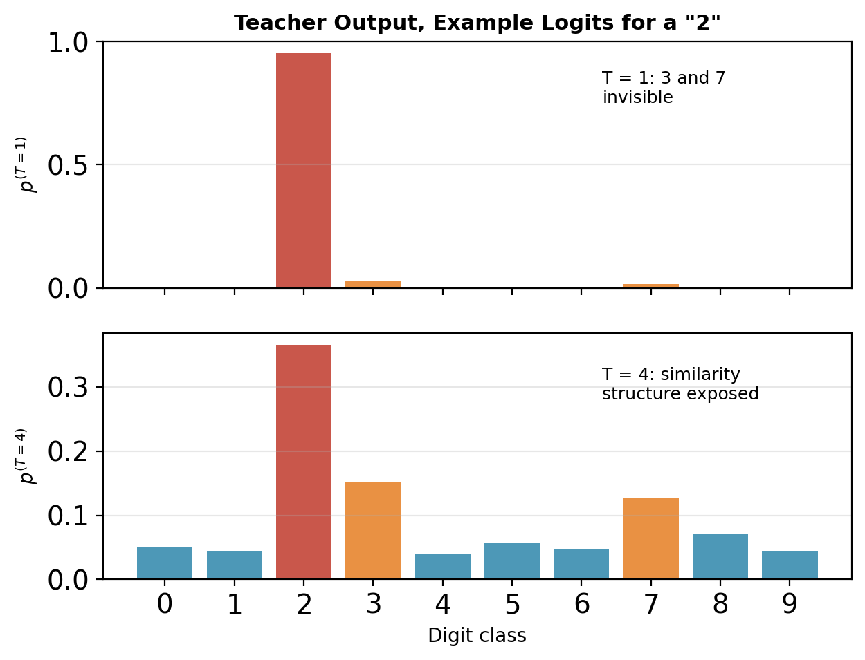
- An image of a 2 gets more teacher mass on 3 and 7 than on 4
- The near-misses encode learned geometry no label provides
At \(T = 1\) this structure is invisible — the correct class takes ~all the mass. Temperature exposes it.
Consequences for the student:
- Every example supervises every class output, not one — more gradient signal per example
- Students train to teacher-level behavior with less data and less capacity
- The student inherits the teacher’s inter-class geometry, not only its decisions
Example logits (right): one handwritten 2, teacher output at two temperatures.
The Techniques Compose
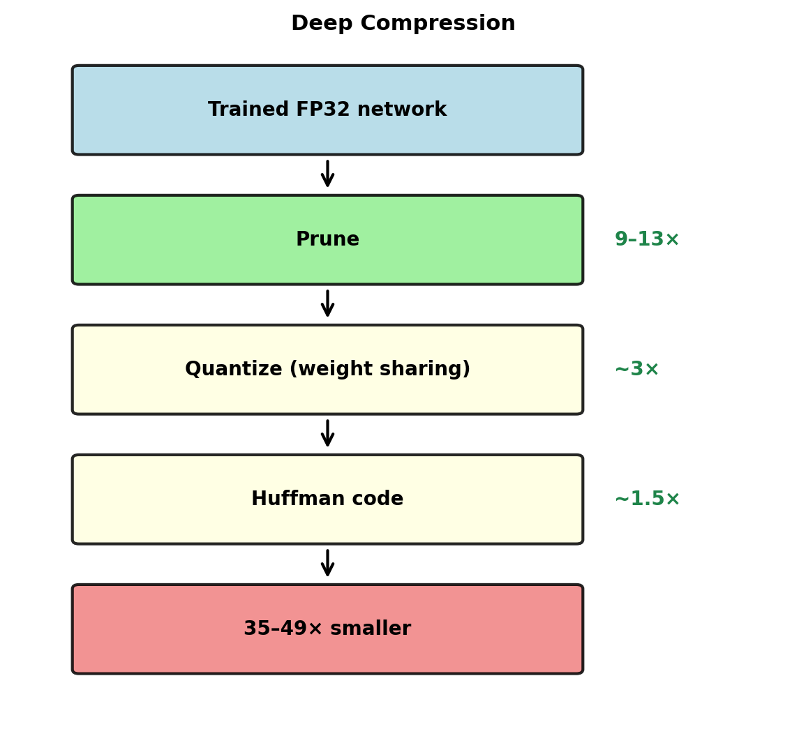
Deep Compression pipeline (Han et al., 2016), applied in sequence:
- Prune — iterative magnitude pruning: 9–13×
- Quantize — k-means weight sharing, 5–8 bits: ~3×
- Entropy-code — Huffman on the indices: ~1.5×
| AlexNet | VGG-16 | |
|---|---|---|
| Original | 240 MB | 552 MB |
| Compressed | 6.9 MB | 11.3 MB |
| Ratio | 35× | 49× |
No accuracy loss on ImageNet.
Interaction limits:
- Pruning and low-bit quantization both degrade weight fidelity — at the extremes the errors compound, the same accumulation as deep PTQ error
- Compressed storage ≠ fast execution: stages 2–3 decompress before compute unless the hardware supports the format
Each Technique Moves the Workload on the Roofline
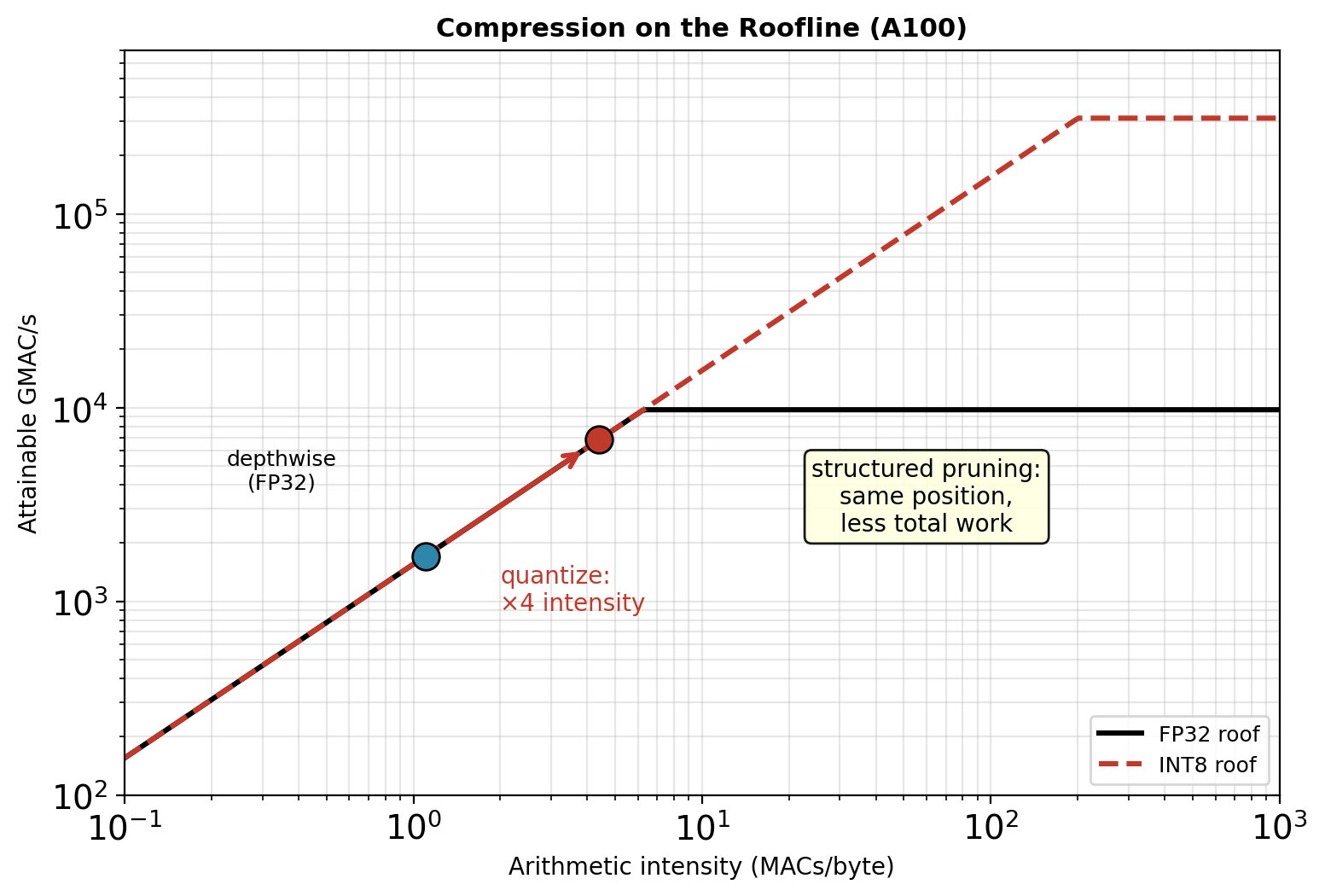
The three techniques on one plot:
Quantization — fewer bytes per value:
- Intensity rises ×4 (INT8): memory-bound layers move up the bandwidth slope
- The roof itself rises with the format’s peak
Structured pruning — fewer values:
- MACs and bytes shrink together: position holds, total work shrinks
- 2:4 doubles the effective peak
Distillation — a smaller model:
- Replaces the workload. The student’s architecture sets the new operating points
Deployment order: distill the capacity, prune the remainder, quantize the result.
Bytes per value, number of values, size of the model: three independent reductions of the same cost.
Learned Features Transfer Across Tasks
Layer Generality
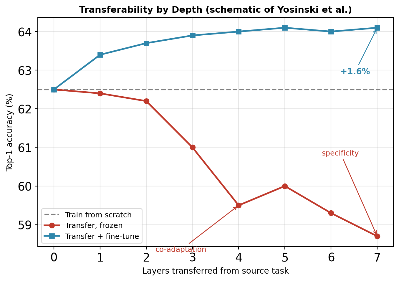
First-layer filters converge to Gabor edges and color blobs regardless of task or dataset (Yosinski et al., 2014).
Specificity increases with depth:
- Layers 1–3: general (edges, textures) — transfer freely
- Layers 4–5: transfer degrades from co-adaptation — fragile joint tuning between neighboring layers
- Layers 6–7: transfer degrades from specificity — features tuned to source classes
Measured Transfer (ImageNet A/B splits)
- Frozen mid-network transfer: up to −4% top-1 vs baseline
- Transfer all layers + fine-tune: +1.6% over training from scratch
Transferred initialization helps even when target data is abundant.