Generative Models: Energy-Based Models and Adversarial Training
EE 641 - Unit 3A
The Deliverable Is New Data
The output of a trained model: samples
- \(\mathbf{x} \sim p_{\boldsymbol{\theta}}\) - new data, not labels or scores
- No per-output ground truth - a generated face matches no training face
- Individually ungradable - only the collection can be judged
The target is a distribution, seen only through samples
- \(p_{\text{data}}\): unknown - available as i.i.d. draws
- Success: \(p_{\boldsymbol{\theta}} \approx p_{\text{data}}\) - the model’s samples collectively indistinguishable from data
The consequence for training
- Objectives become distribution comparisons: forward KL, JS, Wasserstein
- Evaluation becomes distribution comparison too - a sample set against a sample set
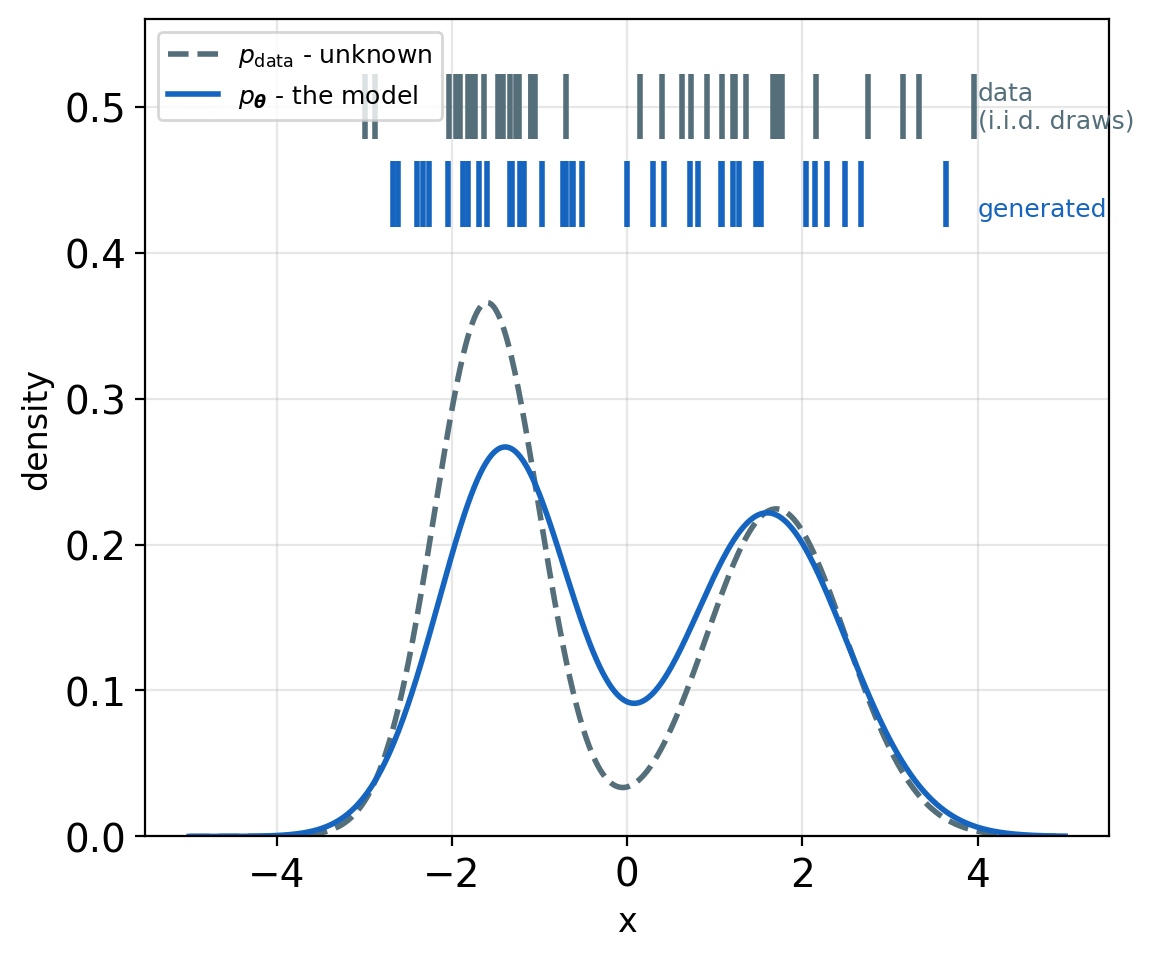
Training and evaluation both compare distributions - the reason divergences run through everything here.
A Density Is a Compressor
Shannon’s link
- An outcome of probability \(p\): codable in \(-\log_2 p\) bits - arithmetic coding achieves it, up to rounding
- Code length under a model: \(-\log_2 p_{\boldsymbol{\theta}}(\mathbf{x})\) bits
- Maximizing log-likelihood ⇔ minimizing the bits to encode the data - the training objective is a compression rate
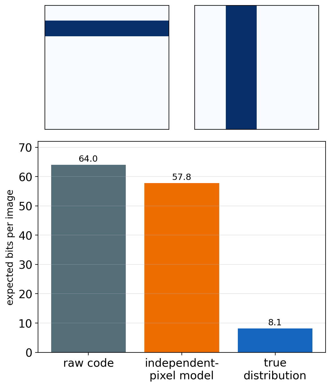
Worked exactly (the figure)
- 8 × 8 binary bar images: raw code = 64 bits
- Per-pixel model (rates fitted, pixels independent): 57.8 bits - marginal rates capture almost nothing
- True distribution: 8.1 bits - orientation + which bars, nothing else to say
- The compression lives entirely in the between-pixel structure - and noise never compresses
Bits per dimension
- Bits per dimension: \(-\log_2 p_{\boldsymbol{\theta}}(\mathbf{x}) / d\) - how image likelihoods are reported
- Learned image densities: ~3 bits/dim on CIFAR-10, against 8 raw
Representing \(p(\mathbf{x})\) requires a functional form - the energy is the most general choice.
The Boltzmann Distribution Converts Energy to Probability
Energy scores configurations
- \(E: \mathbb{R}^d \to \mathbb{R}\), low energy → plausible
\[p(\mathbf{x}) = \frac{1}{Z} \exp\left(-\frac{E(\mathbf{x})}{T}\right), \quad Z = \int \exp\left(-\frac{E(\mathbf{x})}{T}\right) d\mathbf{x}\]
The form follows from maximum entropy
- Maximize \(S = -\sum_i p_i \log p_i\) subject to:
- fixed mean energy: \(\langle E \rangle = U\) (\(\langle \cdot \rangle\) = expectation, used throughout)
- normalization: \(\sum_i p_i = 1\)
- Lagrange multipliers force \(p_i \propto e^{-\beta E_i}\), \(\beta = 1/T\)
No generality lost
- Any positive density: set \(E(\mathbf{x}) = -\log \tilde{p}(\mathbf{x})\)
- Energy determines the distribution completely
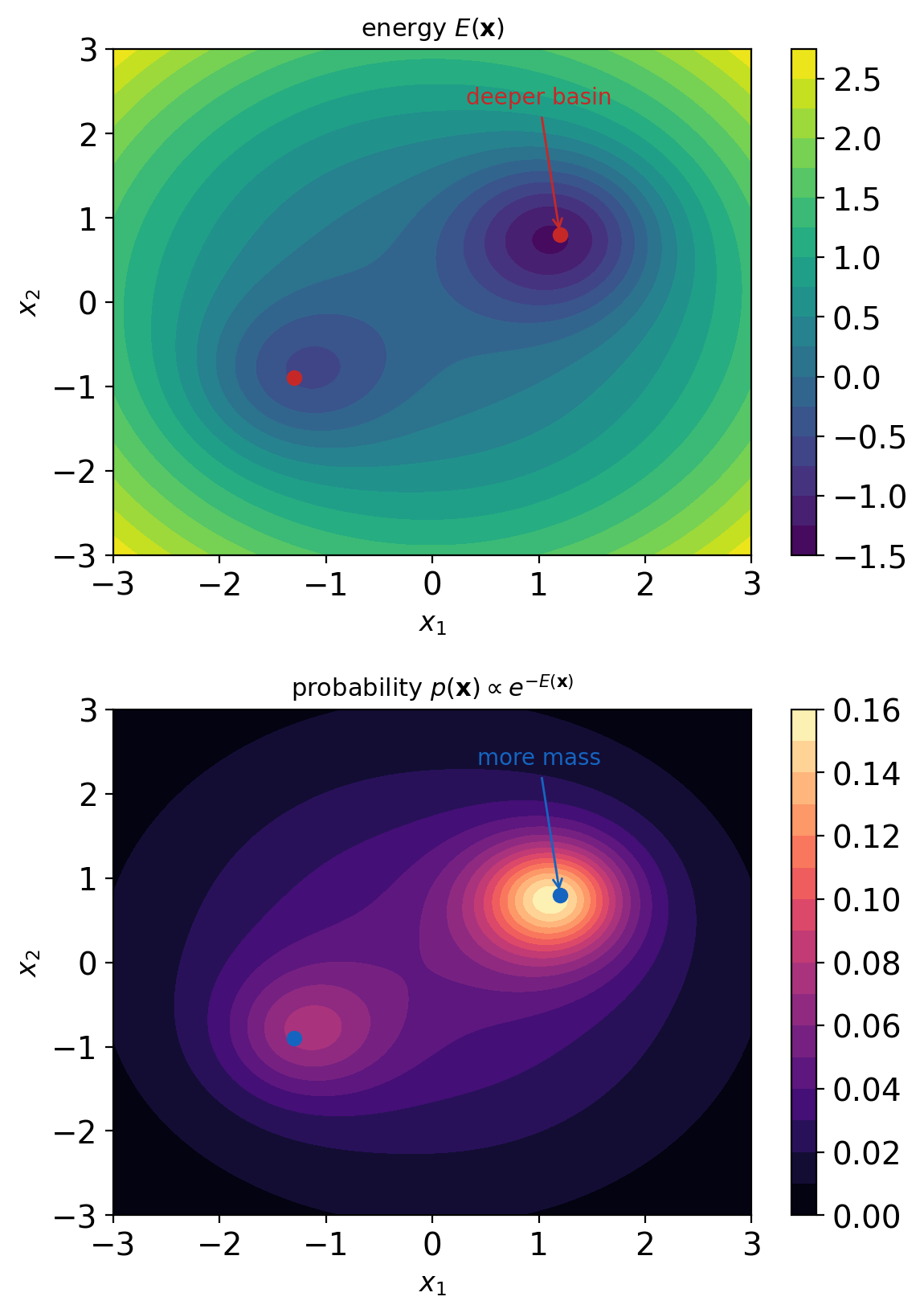
Mass concentrates in low-energy basins - deeper basin, more mass.
Temperature Sets the Concentration Around Minima
\(T\) rescales energy differences - minima unmoved
- \(T \to 0\): mass collapses onto the global minimum - sampling becomes optimization
- \(T \to \infty\): flattens toward uniform
- Intermediate \(T\): sets the mass kept by shallower basins
- Decreasing \(T\) during search: simulated annealing
The score needs no normalization
- \(\nabla_{\mathbf{x}} \log p(\mathbf{x}) = -\frac{1}{T}\nabla_{\mathbf{x}} E(\mathbf{x})\) - differentiating in \(\mathbf{x}\) removes \(\log Z\)
- Log-probability slope: available without \(Z\)
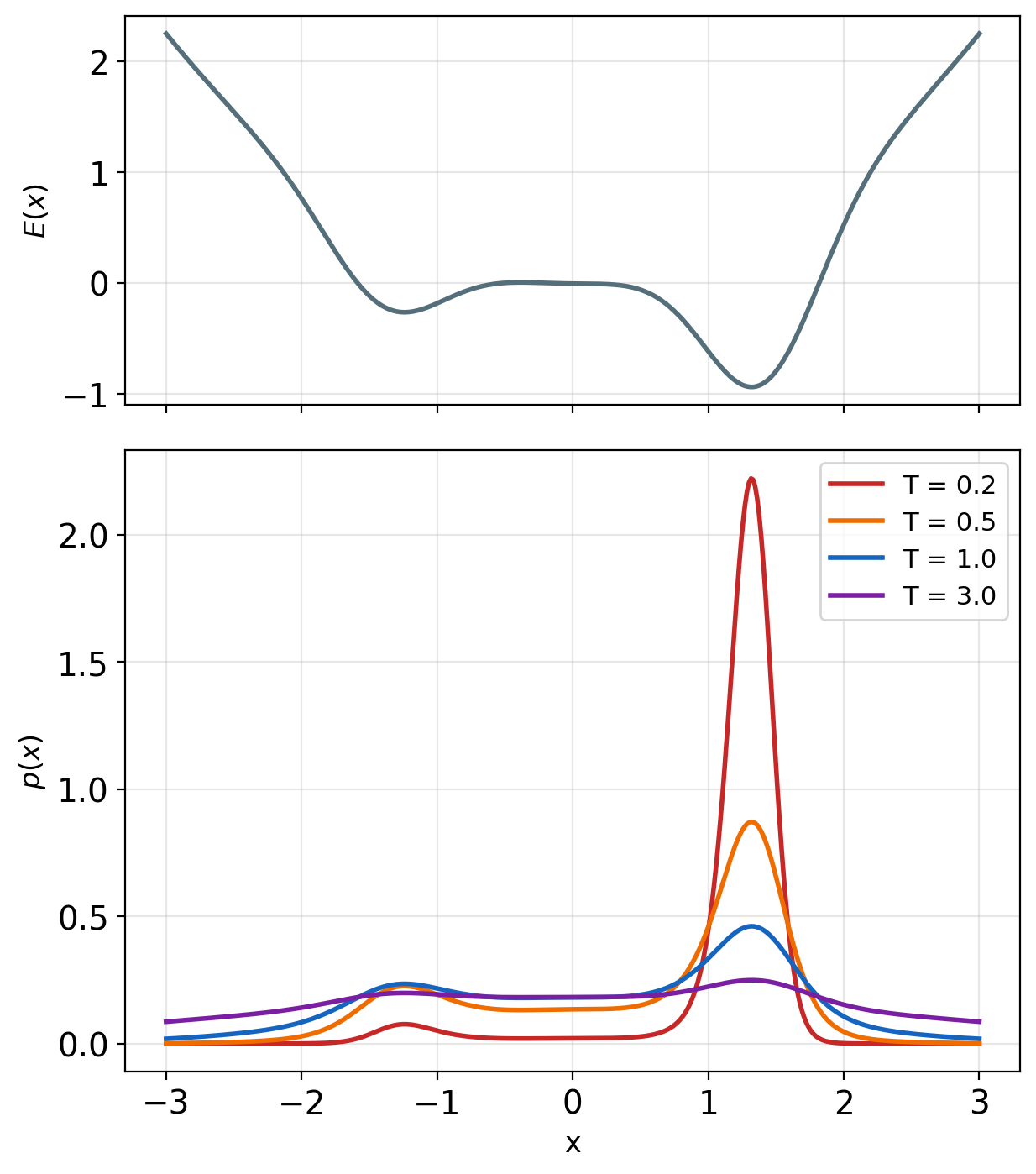
Models fix \(T = 1\) - sampling reintroduces temperature as a control.
Computing Z Is Intractable
\[Z(\boldsymbol{\theta}) = \int \exp(-E(\mathbf{x}; \boldsymbol{\theta}))\, d\mathbf{x}\]
What requires \(Z\)
- Likelihood values: \(\log p(\mathbf{x}) = -E(\mathbf{x}) - \log Z\)
- Model comparison and evaluation
- Training: \(\nabla_{\boldsymbol{\theta}} \log Z\) in every likelihood gradient
What survives without \(Z\)
- Ratios: \(p(\mathbf{x}_1)/p(\mathbf{x}_2) = e^{-(E(\mathbf{x}_1) - E(\mathbf{x}_2))}\)
- The score: \(\nabla_{\mathbf{x}} \log p(\mathbf{x}) = -\nabla_{\mathbf{x}} E(\mathbf{x})\)
- Enough to drive samplers - and score-based training
Counting the terms (binary image, 224 × 224 × 3)
- \(d = 150{,}528\) binary variables: \(Z = \sum_{\mathbf{x} \in \{0,1\}^d} e^{-E(\mathbf{x})}\)
- \(2^{150{,}528} \approx 10^{45{,}313}\) terms
- Atoms in the observable universe: \(\sim 10^{80}\)
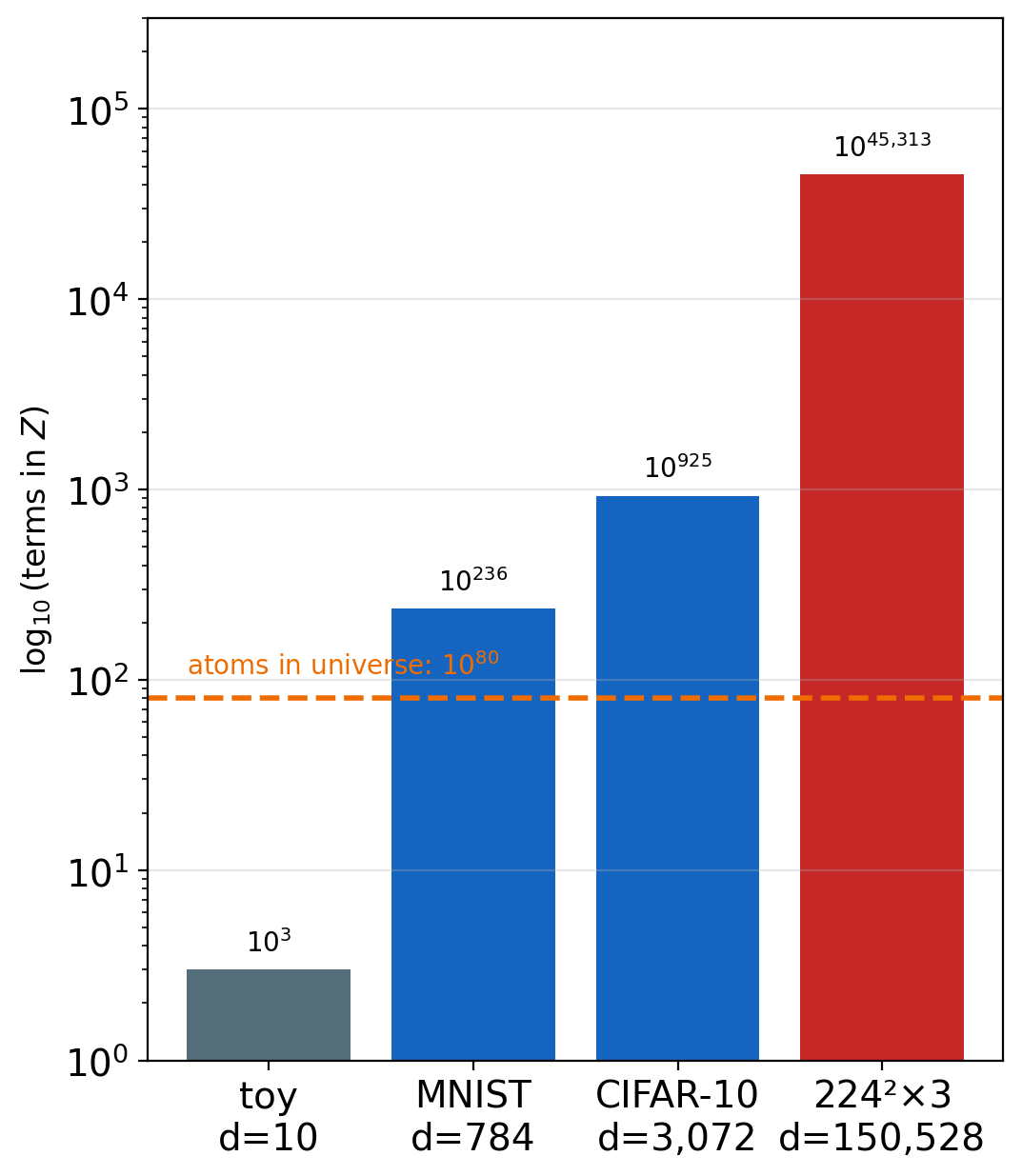
Every EBM training method is a strategy for never evaluating this integral.
Free Energy Derivatives Are Model Expectations
\[F(\boldsymbol{\theta}) = -\log Z(\boldsymbol{\theta}) \qquad (T = 1 \text{ from here on})\]
Differentiate once
\[\frac{\partial F}{\partial \theta_i} = -\frac{1}{Z}\frac{\partial Z}{\partial \theta_i} = \frac{1}{Z}\int e^{-E(\mathbf{x};\boldsymbol{\theta})}\, \frac{\partial E}{\partial \theta_i}\, d\mathbf{x} = \left\langle \frac{\partial E}{\partial \theta_i} \right\rangle_{p(\mathbf{x}|\boldsymbol{\theta})}\]
- One scalar’s derivative = an average under the model
- Physics name: Helmholtz free energy, \(F = U - TS\), minimized at equilibrium
What the identity costs
- Left side: one derivative. Right side: an integral against \(p(\mathbf{x}|\boldsymbol{\theta})\)
- Exact evaluation: as hard as \(Z\)
- Estimation: requires samples from the model
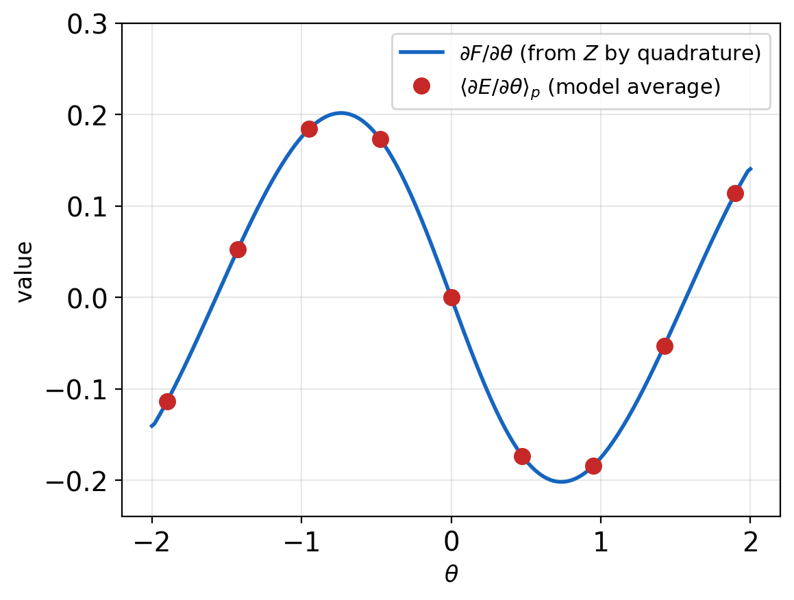
Estimating \(\partial F / \partial \boldsymbol{\theta}\) means sampling from the model - the requirement that shapes all EBM training.
Maximum Likelihood Minimizes Forward KL
Data \(\{\mathbf{x}_1, ..., \mathbf{x}_N\} \sim p_{\text{data}}\):
\[\max_{\boldsymbol{\theta}}\; \mathcal{L}(\boldsymbol{\theta}) = \frac{1}{N}\sum_{i=1}^N \log p(\mathbf{x}_i|\boldsymbol{\theta})\]
The same objective as a divergence
- \(\text{KL}(p \| q) = \mathbb{E}_{p}[\log(p/q)] \geq 0\), zero iff \(p = q\)
- \(N \to \infty\): \(\frac{1}{N}\sum_i \log p_{\boldsymbol{\theta}}(\mathbf{x}_i) \to \mathbb{E}_{p_{\text{data}}}[\log p_{\boldsymbol{\theta}}(\mathbf{x})]\)
- \(\mathbb{E}_{p_{\text{data}}}[\log p_{\boldsymbol{\theta}}] = -\text{KL}(p_{\text{data}} \| p_{\boldsymbol{\theta}}) - H(p_{\text{data}})\), with \(H(p_{\text{data}})\) constant in \(\boldsymbol{\theta}\)
- Max likelihood ⇔ min \(\text{KL}(p_{\text{data}} \| p_{\boldsymbol{\theta}})\) - forward KL, data in the first argument
What forward KL demands
- \(p_{\text{data}} > 0\), \(p_{\boldsymbol{\theta}} \to 0\): integrand \(\to \infty\) - a missed data mode is unboundedly expensive
- \(p_{\text{data}} = 0\): extra model mass costs nothing directly
- Result: cover every mode - spread thin if the family cannot fit all
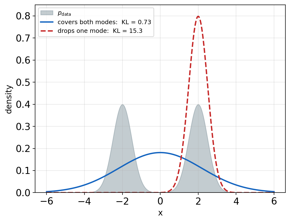
Which divergence a method minimizes determines which errors it tolerates.
The Likelihood Gradient Splits into Two Phases
The objective is a gap
- \(\log p = -E + F\), averaged: \(\mathcal{L}(\boldsymbol{\theta}) = F(\boldsymbol{\theta}) - \langle E \rangle_{\text{data}}\)
- Differentiate, using \(\nabla_{\boldsymbol{\theta}} F = \mathbb{E}_{p}[\nabla_{\boldsymbol{\theta}} E]\):
\[\nabla_{\boldsymbol{\theta}} \log p(\mathbf{x};\boldsymbol{\theta}) = \underbrace{-\nabla_{\boldsymbol{\theta}} E(\mathbf{x};\boldsymbol{\theta})}_{\text{positive phase}} + \underbrace{\mathbb{E}_{p(\mathbf{x}'|\boldsymbol{\theta})}\left[\nabla_{\boldsymbol{\theta}} E(\mathbf{x}';\boldsymbol{\theta})\right]}_{\text{negative phase}}\]
Positive phase - push down at data
- \(\nabla_{\boldsymbol{\theta}} E\) at observed examples - one backward pass each
Negative phase - push up where the model puts mass
- Raises energy where the model concentrates - data or not
- Needs samples from \(p(\mathbf{x}|\boldsymbol{\theta})\) - which changes at every update
Why the \(F\) term must be there
- Without \(F\): \(\max_{\boldsymbol{\theta}} \sum_i -E(\mathbf{x}_i)\) is degenerate - sink all energies, commit mass nowhere
- \(F\) is the counterweight - energy at data counts only relative to everywhere else
- Negative phase = \(\nabla_{\boldsymbol{\theta}} F\), the free-energy gradient - the single intractable term
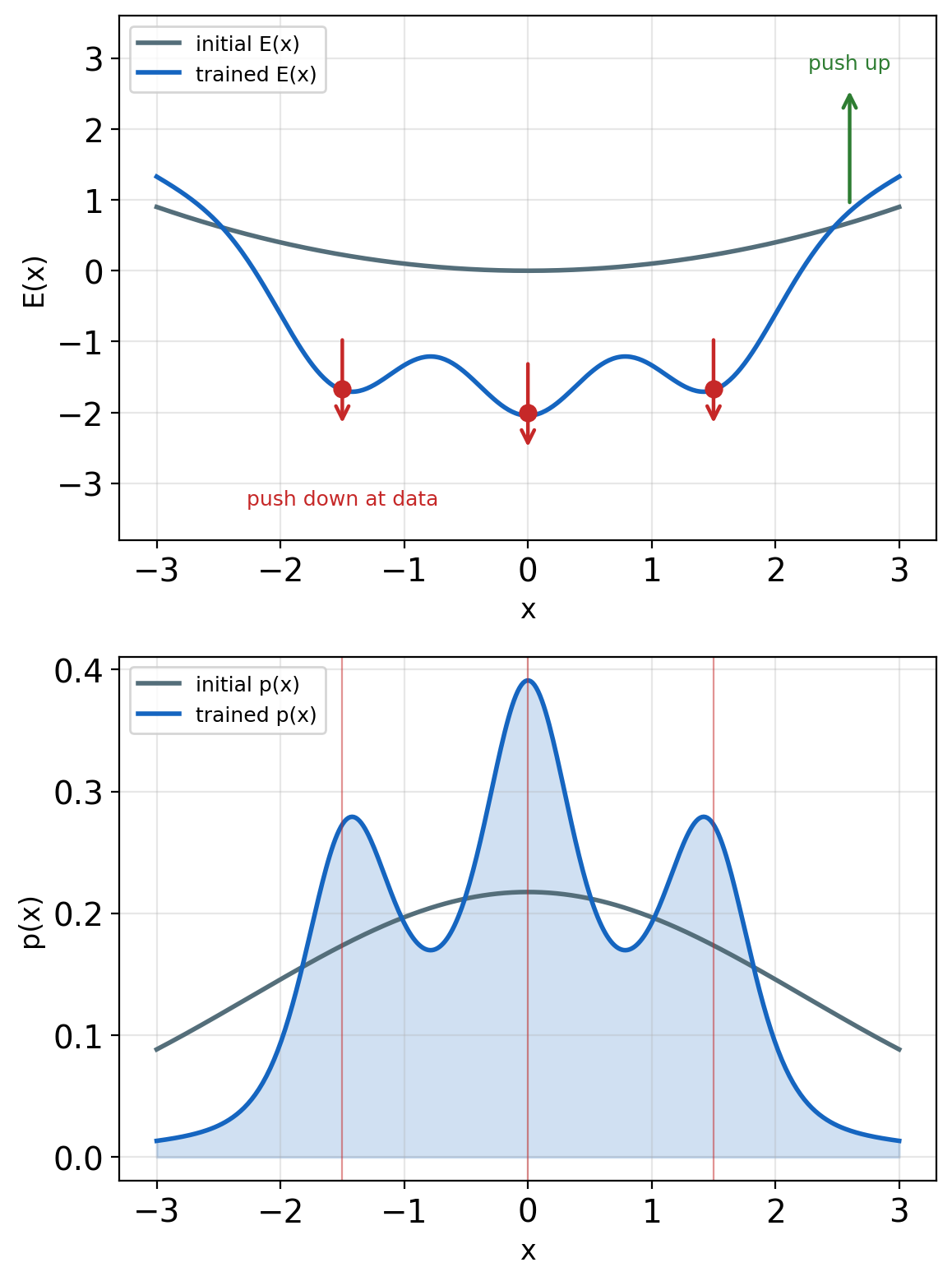
Sampling from the model is the entire difficulty of likelihood training for EBMs.
Training Matches the Statistics the Energy Exposes
At any maximum of the likelihood the two phases balance:
\[\left\langle \nabla_{\boldsymbol{\theta}} E \right\rangle_{\text{data}} = \left\langle \nabla_{\boldsymbol{\theta}} E \right\rangle_{p(\mathbf{x}|\boldsymbol{\theta})}\]
Moment matching
- Feature energy \(E(\mathbf{x}; \boldsymbol{\theta}) = -\boldsymbol{\theta}^\top T(\mathbf{x})\) (exponential family, \(T\) = sufficient statistics): condition becomes \(\langle T(\mathbf{x}) \rangle_{\text{data}} = \langle T(\mathbf{x}) \rangle_{\text{model}}\)
- Matches exactly the statistics the energy exposes - blind to everything outside \(T\)
- The fit: the max-entropy distribution with those statistics - the same principle behind the Boltzmann form
Richer statistics need richer energies
- Hidden variables: extend \(T(\mathbf{x})\) implicitly
- Network energies: learn \(T(\mathbf{x})\)
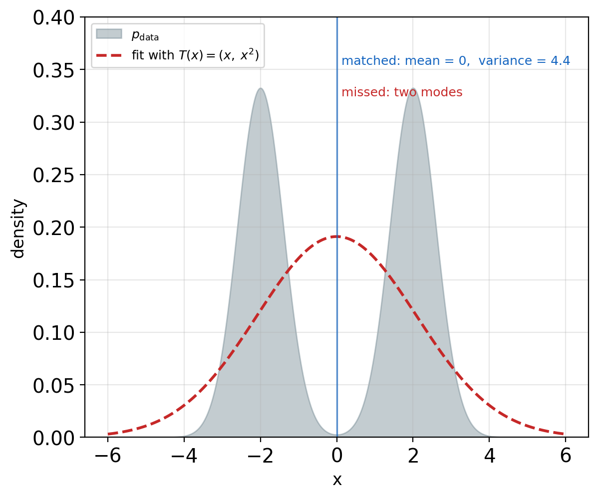
The energy family fixes the statistics the model can represent - the rest is invisible to training.
Sampling Is Not Optimization
Two different asks of the same landscape
- Optimization: \(\arg\max_{\mathbf{x}}\, p(\mathbf{x})\) - one point, the mode (MAP)
- Sampling: visit regions in proportion to their mass - the whole distribution
- The negative phase is an expectation - it needs mass, not modes
The mode is not where the mass is
- Standard Gaussian, \(d\) dimensions: density peaks at \(\mathbf{0}\) - mass concentrates on the shell \(\|\mathbf{x}\| \approx \sqrt{d}\)
- \(d = 100\): no sample ever lands near the mode - the most probable point is not typical
- High dimension: typical set ≠ neighborhood of the mode
One walk, two algorithms
- Deterministic ascent on \(\log p\): parks at a mode - an optimizer
- Matched noise added: visits by mass - a sampler
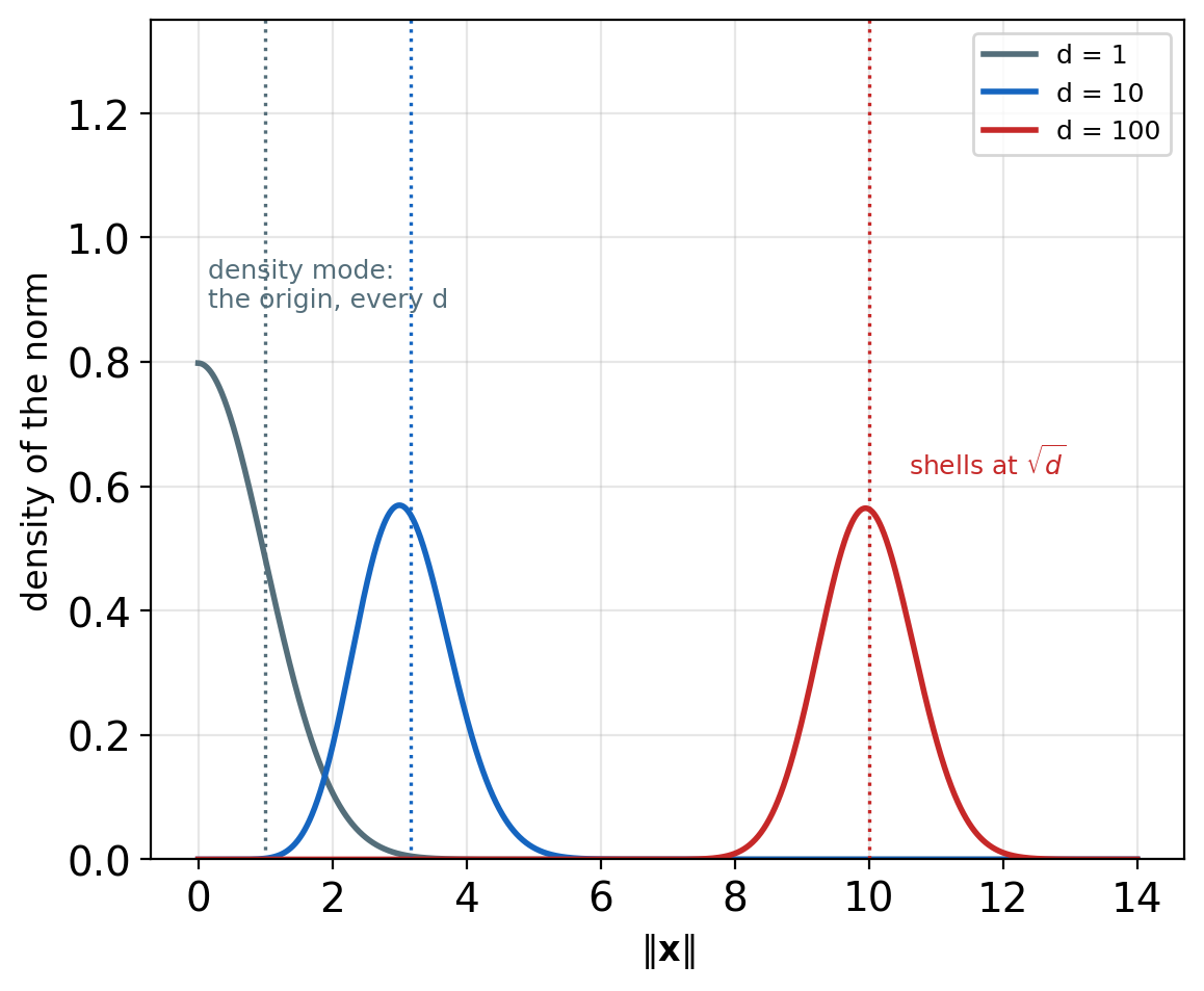
An optimizer answers where probability peaks - a sampler answers where probability lives.
Monte Carlo Shifts the Problem to Sampling
Monte Carlo
- \(\mathbb{E}_{p}[f(\mathbf{x})] \approx \frac{1}{K}\sum_{k=1}^K f(\mathbf{x}^{(k)})\), with \(\mathbf{x}^{(k)} \sim p\)
- Error \(O(1/\sqrt{K})\), dimension-free - for independent samples
- Negative phase: \(f = \nabla_{\boldsymbol{\theta}} E\), \(\;p = p(\mathbf{x}|\boldsymbol{\theta})\)
Producing \(\mathbf{x}^{(k)} \sim p\)
- Direct samplers need more than \(e^{-E}\):
- inverse-CDF: needs the normalized CDF - needs \(Z\)
- rejection sampling: acceptance collapses exponentially in \(d\)
- High-dimensional \(p \propto e^{-E}\): no direct method exists
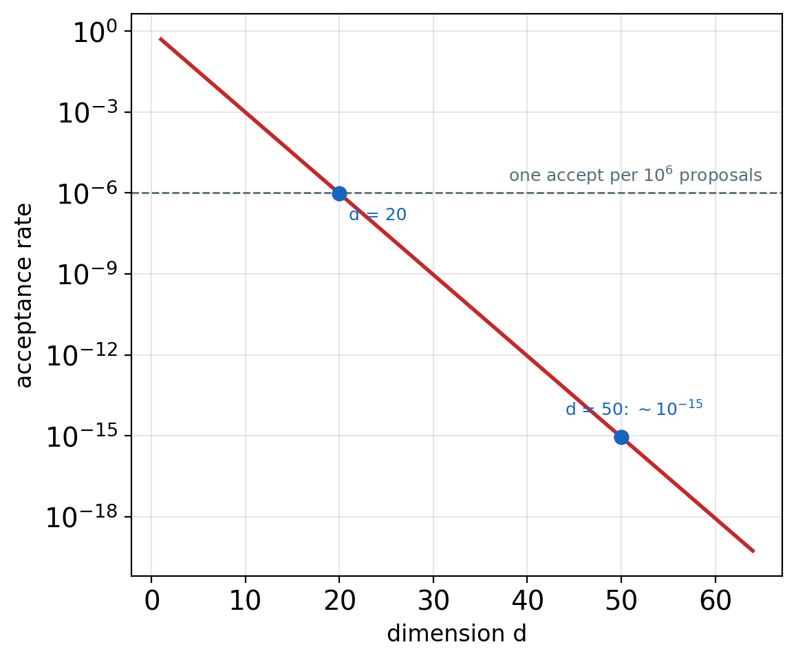
The expectation is easy given samples - producing the samples is the problem.
MCMC Makes the Target the Stationary Distribution
Build the chain around the target
- Known: irreducible + aperiodic → the chain converges to its stationary \(\pi\), from any start
- MCMC reverses it: given target \(p\), build \(T\) with \(\pi = p\)
- Run the chain - its states become the samples
Detailed balance
- \(p(\mathbf{x})\, T(\mathbf{x} \to \mathbf{x}') = p(\mathbf{x}')\, T(\mathbf{x}' \to \mathbf{x})\) \(\Rightarrow\) \(p\) stationary
- Local, checkable - no global computation
Metropolis-Hastings
- Propose \(\mathbf{x}' \sim q(\mathbf{x}'|\mathbf{x})\), accept with \(\min\!\left(1,\; \frac{e^{-E(\mathbf{x}')}\, q(\mathbf{x}|\mathbf{x}')}{e^{-E(\mathbf{x})}\, q(\mathbf{x}'|\mathbf{x})}\right)\)
- Only energy differences - \(Z\) cancels in the ratio
Named kernels
- Metropolis: random-walk proposal + accept/reject
- Gibbs: one block from its exact conditional - always accepted
- Langevin: gradient-informed proposal
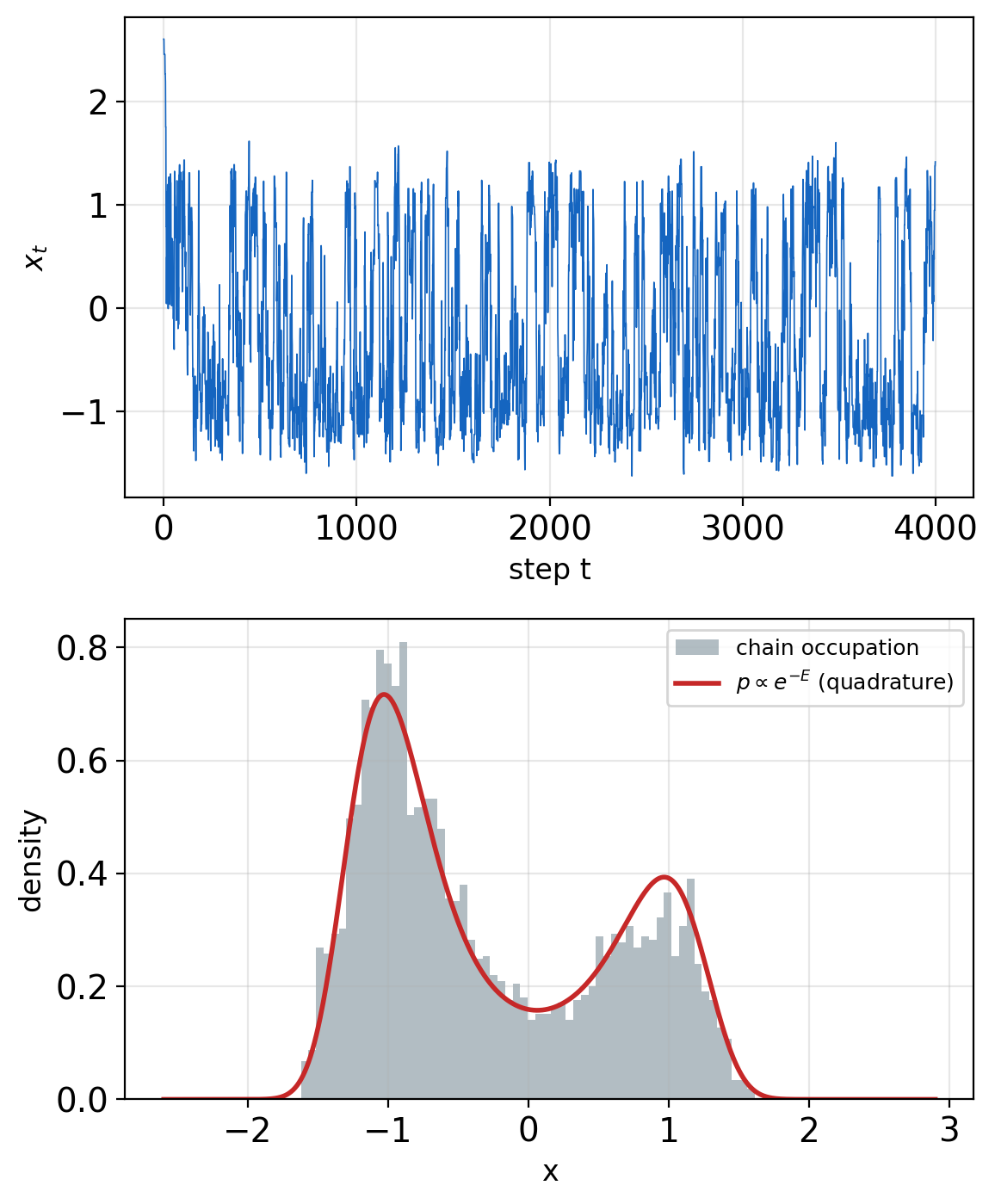
Detailed balance guarantees the target distribution - nothing bounds the time to reach it.
Burn-In and Autocorrelation Set the Sample Budget
Burn-in
- Early states: reflect the start, not \(p\) - the transient toward stationarity
- Standard practice: discard them
Mixing time
- Steps until the chain forgets its start
- Sets the burn-in length - and the spacing between independent-looking states
Autocorrelation
- Successive states dependent - each step adds less than one sample of information
- Effective sample size: \(K_{\text{eff}} = K \,/\, (1 + 2\sum_{t \geq 1} \rho_t)\), \(\;\rho_t\) = lag-\(t\) autocorrelation
- Monte Carlo error: \(O(1/\sqrt{K_{\text{eff}}})\), not \(O(1/\sqrt{K})\)
In practice
- Multiple chains, dispersed starts - agreement diagnoses convergence (\(\hat{R}\))
- No finite test proves stationarity - diagnostics only falsify it
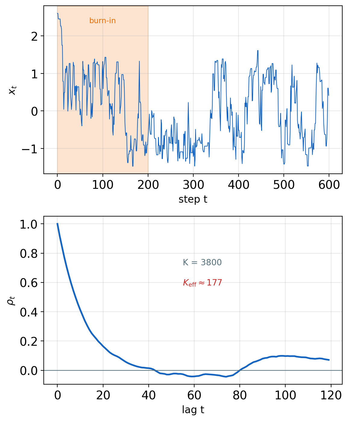
\(K\) chain states are not \(K\) samples - budget by \(K_{\text{eff}}\).
Langevin Dynamics Samples Using Only Energy Gradients
The kernel deep EBMs use in practice - proposals follow the energy gradient
Langevin dynamics
\[\mathbf{x}_{t+1} = \mathbf{x}_t - \frac{\epsilon}{2}\nabla_{\mathbf{x}} E(\mathbf{x}_t) + \sqrt{\epsilon}\,\boldsymbol{\eta}_t, \qquad \boldsymbol{\eta}_t \sim \mathcal{N}(0, \mathbf{I})\]
- Drift = the score: \(\frac{\epsilon}{2}\,\mathbf{s}(\mathbf{x})\), \(\;\mathbf{s} = -\nabla_{\mathbf{x}} E\) - a small step uphill on \(\log p\)
- Noise on, scales matched (\(\epsilon/2\) drift, \(\sqrt{\epsilon}\) noise): stationary distribution exactly \(p \propto e^{-E}\) as \(\epsilon \to 0\)
- Noise is not a nuisance - it is what makes the walk a sampler rather than an optimizer
- Finite \(\epsilon\): discretization bias - a Metropolis correction fixes it (MALA)
Hamiltonian Monte Carlo
- Auxiliary momentum \(\mathbf{p} \sim \mathcal{N}(0, \mathbf{M})\), simulate \(H(\mathbf{x},\mathbf{p}) = E(\mathbf{x}) + \frac{1}{2}\mathbf{p}^\top\mathbf{M}^{-1}\mathbf{p}\)
- Long coherent moves + Metropolis correction - fewer, longer steps
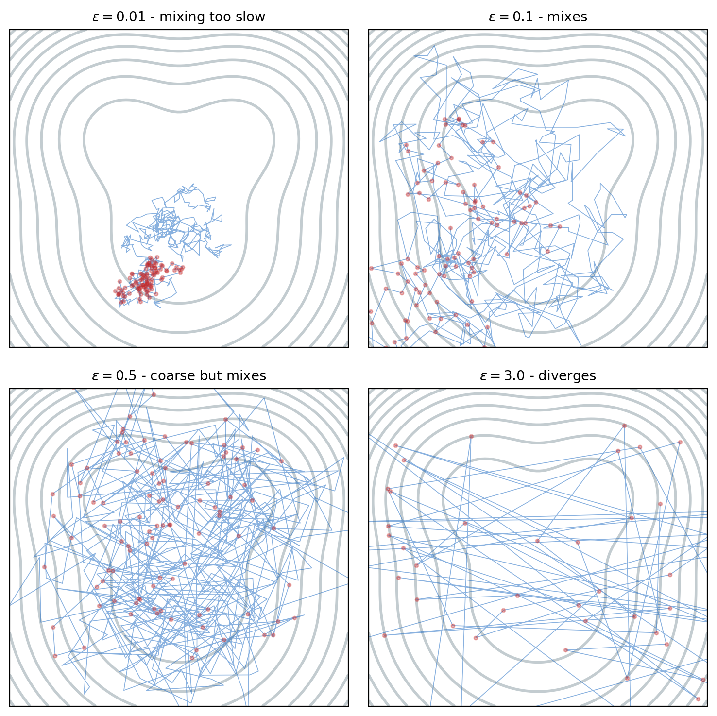
Step size trades discretization error against exploration - no setting fixes separated modes.
Energy Barriers Make Mixing Exponentially Slow
Escaping a basin is a rare event
- Barrier of height \(\Delta E\): crossing fluctuation has probability \(\propto e^{-\Delta E / T}\) per attempt
- Expected escape time (Kramers): \(\tau \sim e^{\Delta E / T}\) - exponential in barrier height
High dimension compounds it
- Image modes: far apart, separated by wide near-zero-probability regions
- Stable \(\epsilon\) capped by the steepest curvature - higher \(d\) → smaller steps, more of them
Spectral view
- Kernel eigenvalues \(1 = \lambda_1 > |\lambda_2| \geq \dots\): mixing time \(\sim 1/(1 - |\lambda_2|)\)
- Deep barrier → \(|\lambda_2| \to 1\): two near-invariant sets (metastability)
- Kramers’ \(e^{\Delta E/T}\) = the spectral gap closing - a property of the landscape, not the budget
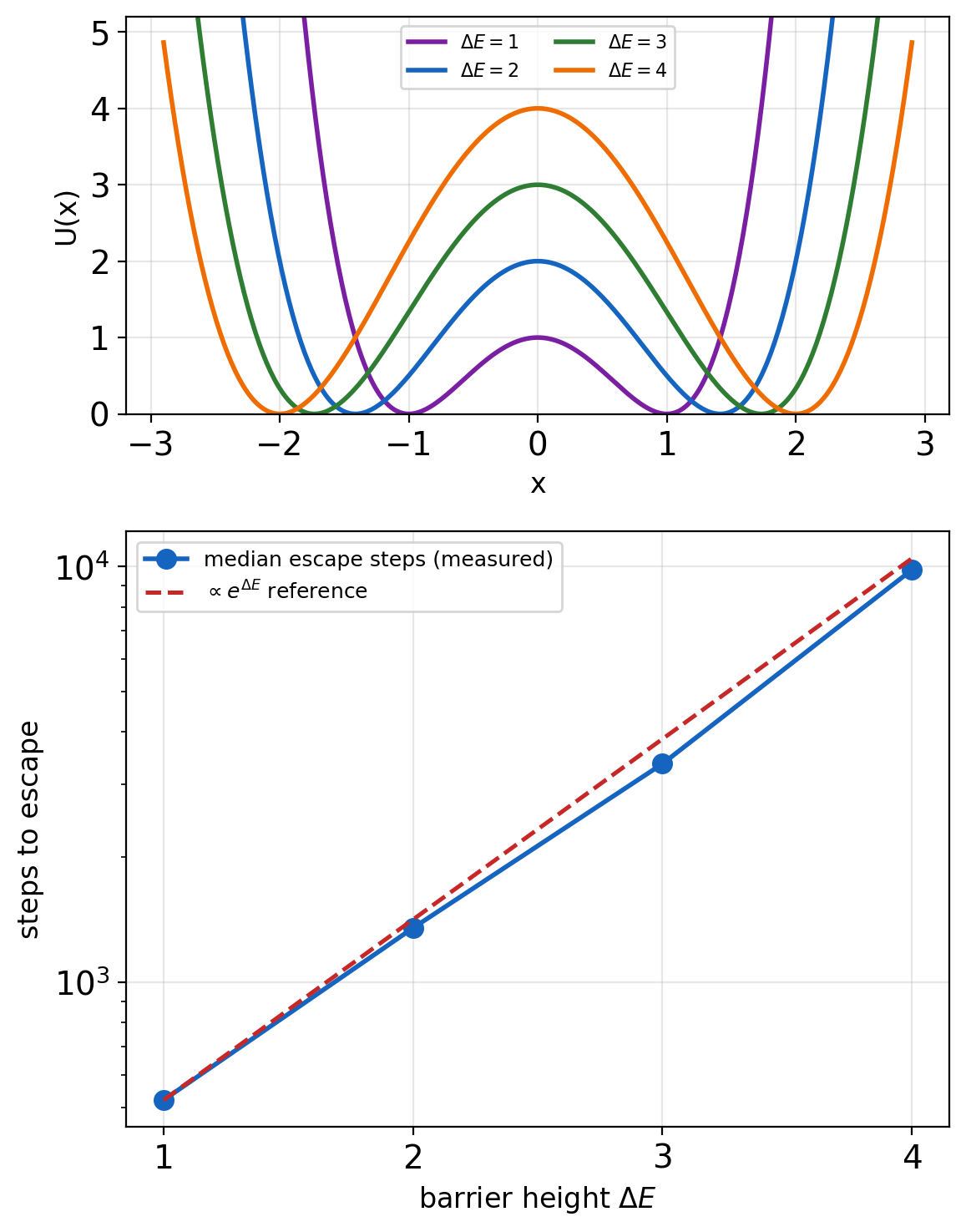
At image scale the chain never reaches the distribution the gradient formula assumes.
“Restricted” Means No Within-Layer Edges
Boltzmann machine (Ackley, Hinton, Sejnowski 1985)
- Binary units, every pair connected: \(E(\mathbf{x}) = -\mathbf{x}^\top \mathbf{J}\, \mathbf{x} - \mathbf{b}^\top \mathbf{x}\)
- Undirected graphical model: edge = direct pairwise interaction
- Gibbs sampling: one unit at a time, each conditioned on all its neighbors
The restriction
- Split the units: visible \(\mathbf{v}\) (the data) and hidden \(\mathbf{h}\) (latent)
- Delete every within-layer edge - “restricted” names exactly this deletion
- Bipartite graph: interactions between layers only
What a deleted edge means
- No edge → no direct interaction → conditional independence given the other layer
- Graph separation as the Markov property - on a graph instead of a chain
- Visible-visible structure: not lost - routed through shared hidden units
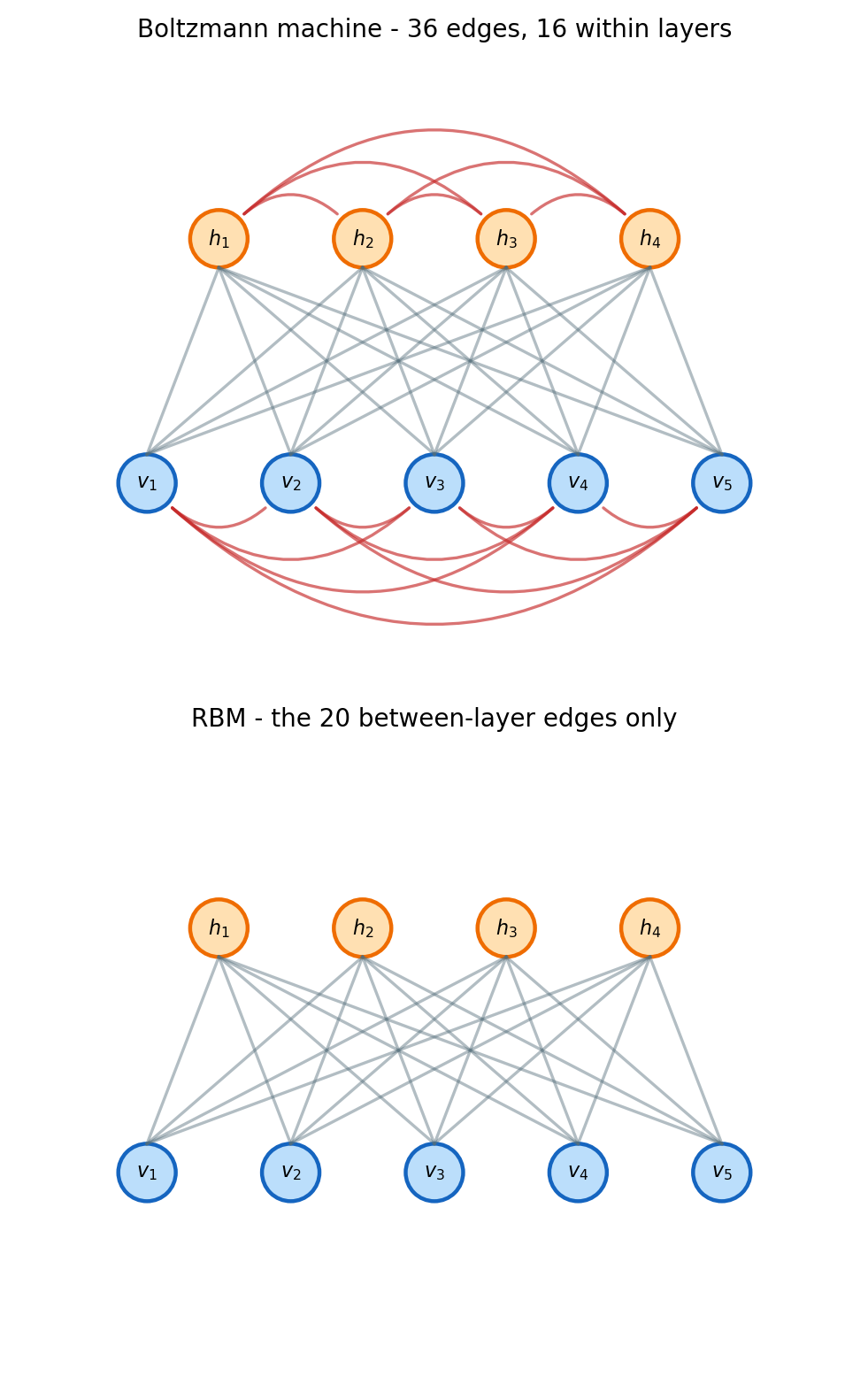
Deleting edges is what turns unit-at-a-time Gibbs into two block draws.
Visible Units Are the Data
What the units are
- \(\mathbf{v}\) = the data vector, componentwise - binary MNIST: 784 visible units, \(v_i\) = pixel \(i\)
- \(\mathbf{h}\) = auxiliary variables - no pixel meaning, only induced dependencies among \(\mathbf{v}\)
- Trained: each hidden unit → a feature detector, a learned pattern over pixels
The data model is the marginal
\[p(\mathbf{v}) = \frac{1}{Z} \sum_{\mathbf{h}} e^{-E(\mathbf{v}, \mathbf{h})}\]
- The same Boltzmann machinery, instantiated on pixels, hidden units integrated out
- Training: the two-phase gradient, on this graph
- Sampling an image: block Gibbs, on this graph
Role
- The first EBM trained at useful scale: MNIST features, deep belief networks (Hinton 2002-2006)
- Surviving in 2026: the concepts, not the model - CD → deep energy models, hidden units → latent variables
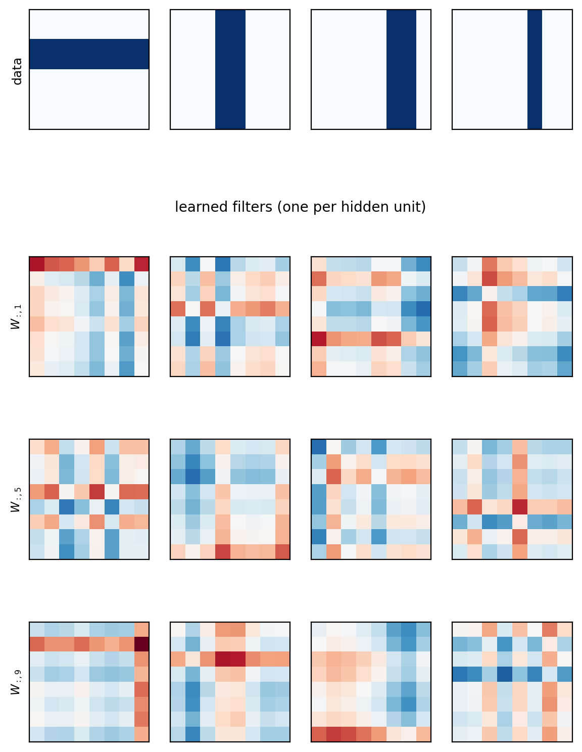
Hidden units are a first appearance of latent variables - VAEs make them continuous and learn the inference.
Bipartite Structure Makes Gibbs Sampling Tractable
Bipartite energy
\[E(\mathbf{v}, \mathbf{h}) = -\mathbf{v}^\top \mathbf{W} \mathbf{h} - \mathbf{b}^\top \mathbf{v} - \mathbf{c}^\top \mathbf{h}\]
- Visible \(\mathbf{v} \in \{0,1\}^D\), hidden \(\mathbf{h} \in \{0,1\}^H\)
- Connections between layers only - none within
Fix \(\mathbf{v}\) - the energy regroups
\[E(\mathbf{v}, \mathbf{h}) = -\mathbf{b}^\top \mathbf{v} - \sum_{j=1}^{H} h_j \left( \mathbf{W}_{:,j}^\top \mathbf{v} + c_j \right)\]
- One term per \(h_j\), no cross terms - the deleted edges are the missing cross terms
- \(e^{-E}\) factorizes over \(j\) → each binary factor normalizes to a sigmoid
Conditionals
\[p(h_j = 1|\mathbf{v}) = \sigma(\mathbf{W}_{:,j}^\top \mathbf{v} + c_j), \qquad p(v_i = 1|\mathbf{h}) = \sigma(\mathbf{W}_{i,:}\, \mathbf{h} + b_i)\]
- \(p(\mathbf{h}|\mathbf{v}) = \prod_j p(h_j|\mathbf{v})\) - and symmetrically for \(\mathbf{v}\) given \(\mathbf{h}\)
- \(p(\mathbf{h}|\mathbf{v})\): exactly a sigmoid layer - a familiar network object
Block Gibbs sampling
- All of \(\mathbf{h}\) in one parallel draw, then all of \(\mathbf{v}\) - one matrix multiply each
- Unrestricted machine: \(h\)-\(h\) edges couple the hiddens - \(p(\mathbf{h}|\mathbf{v})\) does not factorize, Gibbs goes one unit at a time
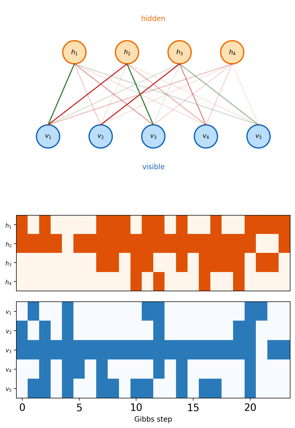
Tractable conditionals - the negative phase still needs the chain to mix.
Contrastive Divergence Truncates the Negative Phase
CD-k
- Start at data: \(\mathbf{v}^{(0)} = \mathbf{x}_{\text{data}}\)
- Alternate: \(\mathbf{h}^{(t)} \sim p(\mathbf{h}|\mathbf{v}^{(t)})\), then \(\mathbf{v}^{(t+1)} \sim p(\mathbf{v}|\mathbf{h}^{(t)})\)
- After \(k\) rounds: \((\mathbf{v}^{(k)}, \mathbf{h}^{(k)})\) = the stand-in model sample
Gradient estimate
\[\Delta \mathbf{W} \propto \langle \mathbf{v}\mathbf{h}^\top \rangle_{\text{data}} - \langle \mathbf{v}\mathbf{h}^\top \rangle_{k}\]
- Visible-hidden correlation matching, truncated at \(k\) steps
- Bias: \(\langle \cdot \rangle_k \neq \langle \cdot \rangle_{\text{model}}\) for every finite \(k\)
- CD-1: the standard choice in practice (Hinton 2002)
- No burn-in, no equilibrium wait - \(k\) steps, total
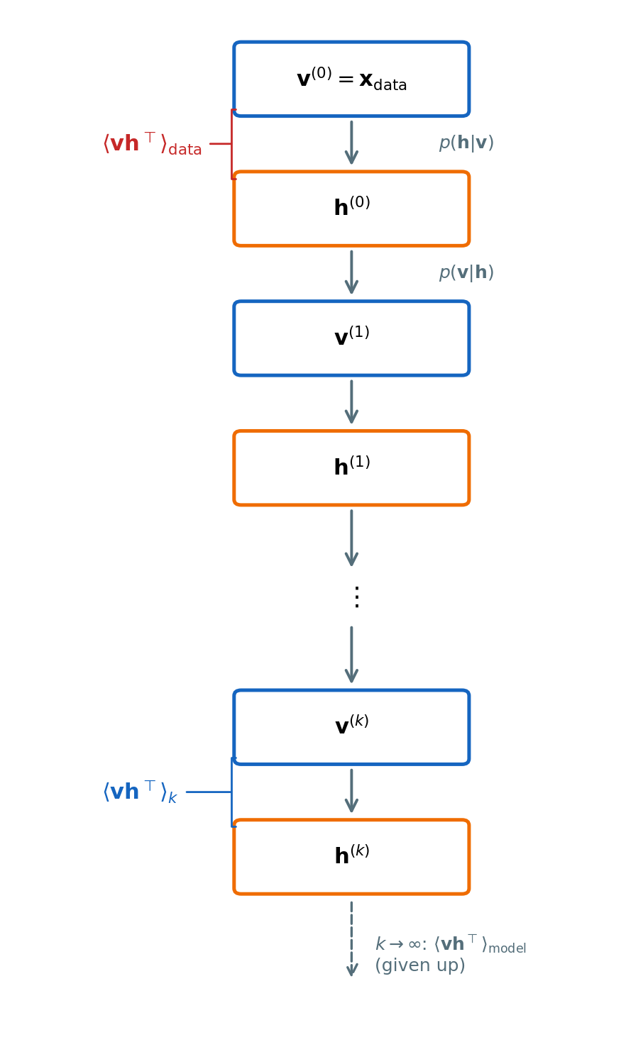
Chains start at the data - the estimate stays near the data distribution.
CD Optimizes a Difference of Divergences
Objective (Hinton 2002)
\[\text{CD}_k = \text{KL}(p_{\text{data}} \| p_{\text{model}}) - \text{KL}(p_k \| p_{\text{model}})\]
- \(p_k\): distribution after \(k\) Gibbs steps from the data
- Not maximum likelihood - the second term is the truncation
Why the gradient is tractable
\[\frac{\partial\, \text{CD}_k}{\partial \boldsymbol{\theta}} \approx \mathbb{E}_{p_{\text{data}}}\!\left[\nabla_{\boldsymbol{\theta}} E\right] - \mathbb{E}_{p_k}\!\left[\nabla_{\boldsymbol{\theta}} E\right]\]
- The \(\nabla_{\boldsymbol{\theta}} \log Z\) terms cancel between the two KLs - no equilibrium sampling anywhere
- Third term (\(\partial p_k / \partial \boldsymbol{\theta}\)): dropped - empirically negligible (Hinton 2002)
Consequences
- \(p_k\) starts at the data → data manifold learned quickly
- Between-mode regions: poorly modeled - spurious modes possible
- Persistent CD: chains continue across minibatches - less bias, more computation
- CD-1 ≈ score matching at the data (Hyvärinen 2007)
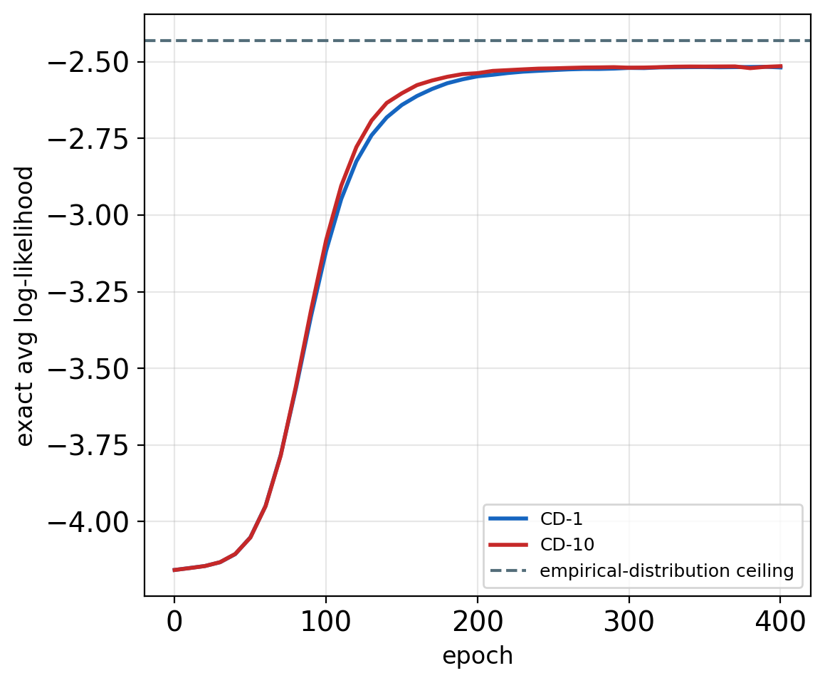
A biased estimator, cheap enough to make RBM training practical.
Score Matching Removes Z from the Objective
Fit the score, not the density
- Score: \(\mathbf{s}(\mathbf{x}; \boldsymbol{\theta}) = \nabla_{\mathbf{x}} \log p(\mathbf{x}; \boldsymbol{\theta})\)
- For an EBM: \(\mathbf{s}(\mathbf{x}) = -\nabla_{\mathbf{x}} E(\mathbf{x}; \boldsymbol{\theta})\) - no \(Z\) anywhere
\[J(\boldsymbol{\theta}) = \tfrac{1}{2}\,\mathbb{E}_{p_{\text{data}}}\!\left[\|\mathbf{s}(\mathbf{x}; \boldsymbol{\theta}) - \nabla_{\mathbf{x}} \log p_{\text{data}}(\mathbf{x})\|^2\right]\]
\(\nabla_{\mathbf{x}} \log p_{\text{data}}\) is unknown
- Integration by parts removes it (Hyvärinen 2005):
\[J(\boldsymbol{\theta}) = \mathbb{E}_{p_{\text{data}}}\!\left[\text{tr}\!\left(\nabla_{\mathbf{x}} \mathbf{s}(\mathbf{x}; \boldsymbol{\theta})\right) + \tfrac{1}{2}\|\mathbf{s}(\mathbf{x}; \boldsymbol{\theta})\|^2\right] + C\]
- Data samples only - no model samples, no MCMC
What the trace term costs
- \(\text{tr}(\nabla_{\mathbf{x}} \mathbf{s})\): \(d\) Hessian-diagonal entries - one backward pass per dimension
- Images (\(d \sim 10^5\)): the objective itself becomes the bottleneck
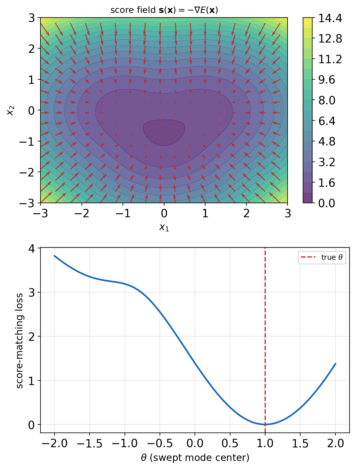
Sampling is gone - the trace term takes its place as the obstacle.
Denoising Makes Score Matching Practical
Perturb, then regress
- Noisy copies: \(\tilde{\mathbf{x}} = \mathbf{x} + \boldsymbol{\epsilon}\), \(\;\boldsymbol{\epsilon} \sim \mathcal{N}(0, \sigma^2 \mathbf{I})\)
- Known conditional score: \(\nabla_{\tilde{\mathbf{x}}} \log p(\tilde{\mathbf{x}}|\mathbf{x}) = -\frac{\tilde{\mathbf{x}} - \mathbf{x}}{\sigma^2}\)
Equivalence (Vincent 2011)
\[\mathbb{E}\!\left[\left\|\mathbf{s}(\tilde{\mathbf{x}}) - \nabla_{\tilde{\mathbf{x}}} \log p(\tilde{\mathbf{x}}|\mathbf{x})\right\|^2\right] = \mathbb{E}\!\left[\left\|\mathbf{s}(\tilde{\mathbf{x}}) + \frac{\tilde{\mathbf{x}} - \mathbf{x}}{\sigma^2}\right\|^2\right] + C\]
- A regression target replaces the trace term - one forward pass per example
Denoising autoencoder connection
- Predicting \(\mathbf{x} - \tilde{\mathbf{x}}\) = learning the score: network output \(= \sigma^2\, \mathbf{s}(\tilde{\mathbf{x}})\)
- Denoising is score estimation
Basis of diffusion models
- Multiple noise levels → annealed score matching
- Learn \(\mathbf{s}(\mathbf{x}, t)\) across noise scales \(\sigma_t\) - the basis of DDPM and score-based models
- A learned score dropped into the Langevin walk = a sampler with no energy anywhere - how score-based models generate
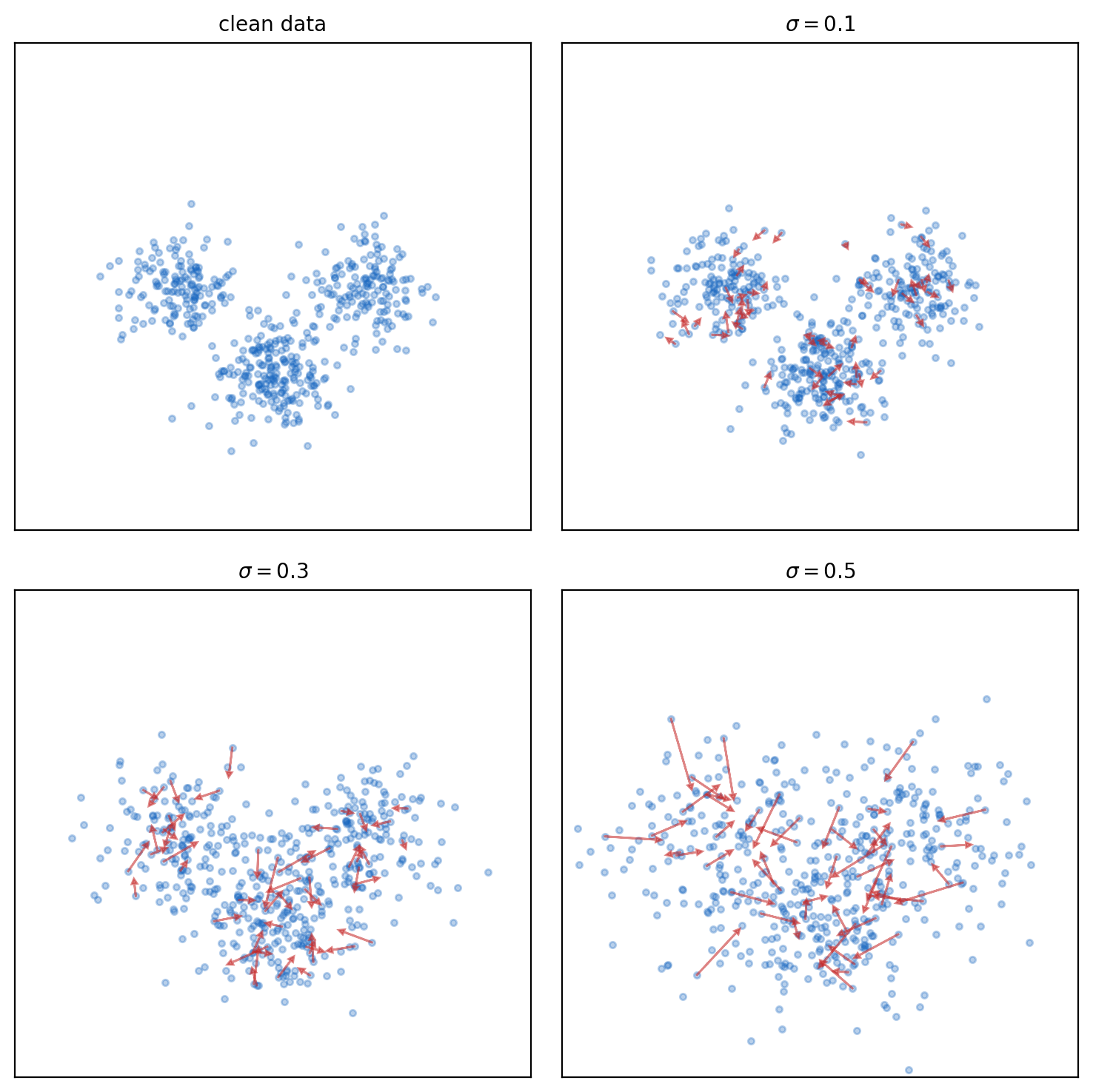
The trace term is gone too - denoising regression needs only forward passes on noisy data.
A Network Energy Trains by Short-Run Langevin
Energy parameterizations
- Direct: \(E(\mathbf{x}; \boldsymbol{\theta}) = f_{\boldsymbol{\theta}}(\mathbf{x})\), a network with scalar output
- From a classifier: \(E(\mathbf{x}) = -\log \sum_y e^{f_{\boldsymbol{\theta}}(\mathbf{x}, y)}\) - logits define an energy
Training loop (sketch)
Budget (Du and Mordatch 2019)
- 60 Langevin steps per negative sample, replay buffer of 10,000 images
- Memory: buffer + per-step sampling gradients - well above a discriminative model’s
- Chains nowhere near equilibrium - the CD trade at network scale
Persistent problems
- Mode coverage poor - short chains inherit the mixing limits
- Training unstable at high capacity
- Sampling stays expensive: 60+ gradient evaluations per image
- Evaluation without likelihoods: unresolved
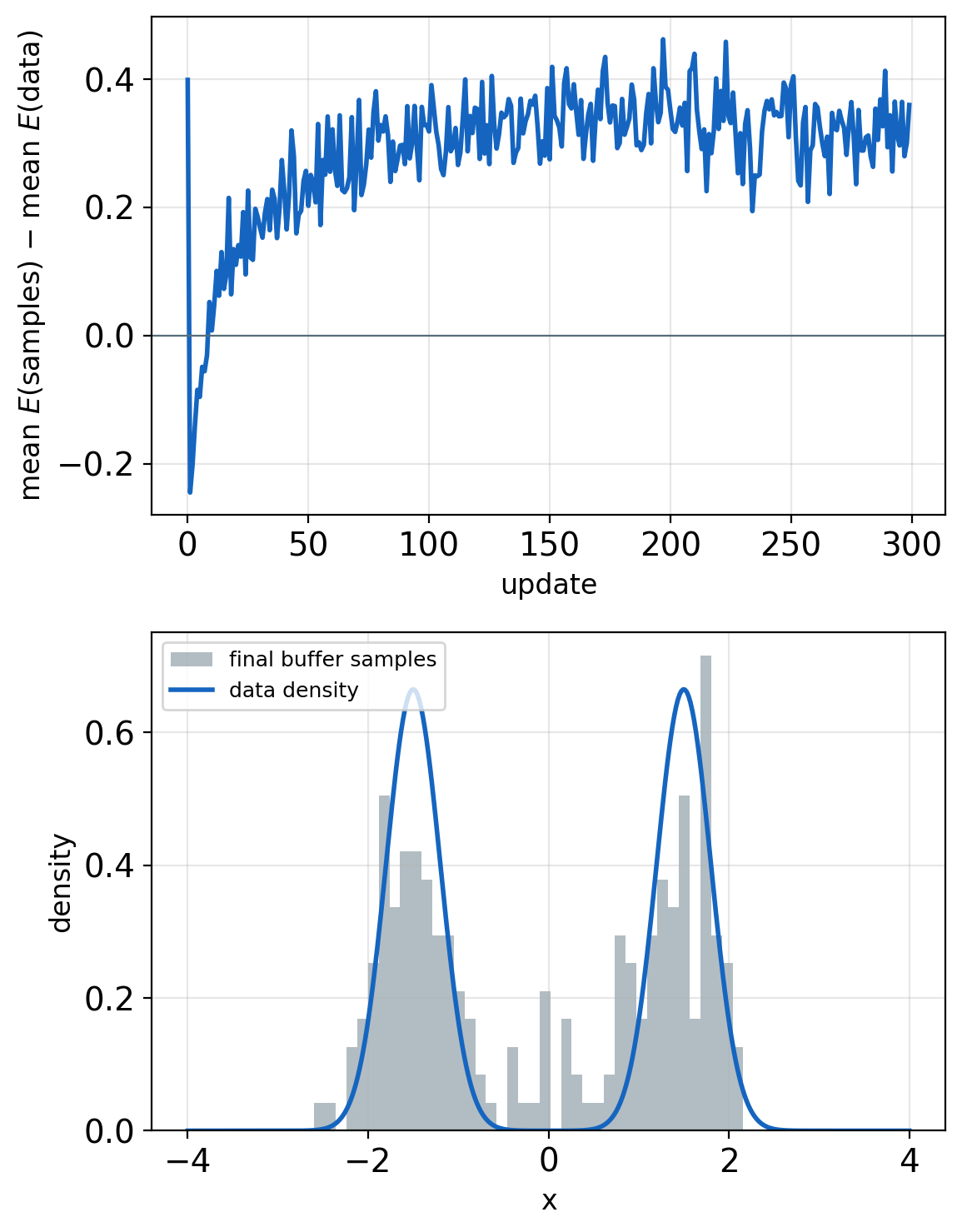
A network energy is learned statistics - \(T(\mathbf{x})\) with millions of parameters.
Why EBMs Failed at Scale
Cost per update, at the published truncation
- 60 Langevin steps per negative sample (Du and Mordatch 2019)
- Each step: one forward + one backward → ~120 network evaluations per sample
- Discriminative update: 2 - a factor of ~60, before any bias correction
- Unbiased training: no finite budget - escape times scale as \(e^{\Delta E}\)
Memory
- Replay buffer: 10,000 persistent sample images
- Sampling gradients at every Langevin step, on top of the parameter gradients
Beyond computation
- High-dimensional spaces: almost entirely empty
- Modes separated by wide near-zero-probability regions
- Local moves cannot cross them - the landscape, not the hardware
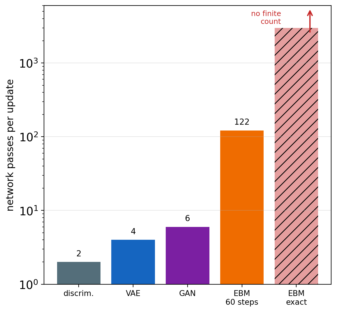
Truncated training runs ~60× a classifier’s cost - unbiased training has no finite cost at all.
What Survived from EBMs
Score matching → diffusion models
- Denoising score matching across noise scales
- DDPM and score-based models - the dominant image generators
Contrastive ideas → self-supervised learning
- InfoNCE ← noise-contrastive estimation, an EBM training method
- SimCLR, MoCo: positive pairs pushed down, negatives pushed up
- CLIP: a contrastive objective over image-text pairs
Around the intractability → the other families
- GANs: drop the density, keep the sampler
- VAEs: bound the likelihood
- Normalizing flows: architectures with \(Z = 1\) by construction
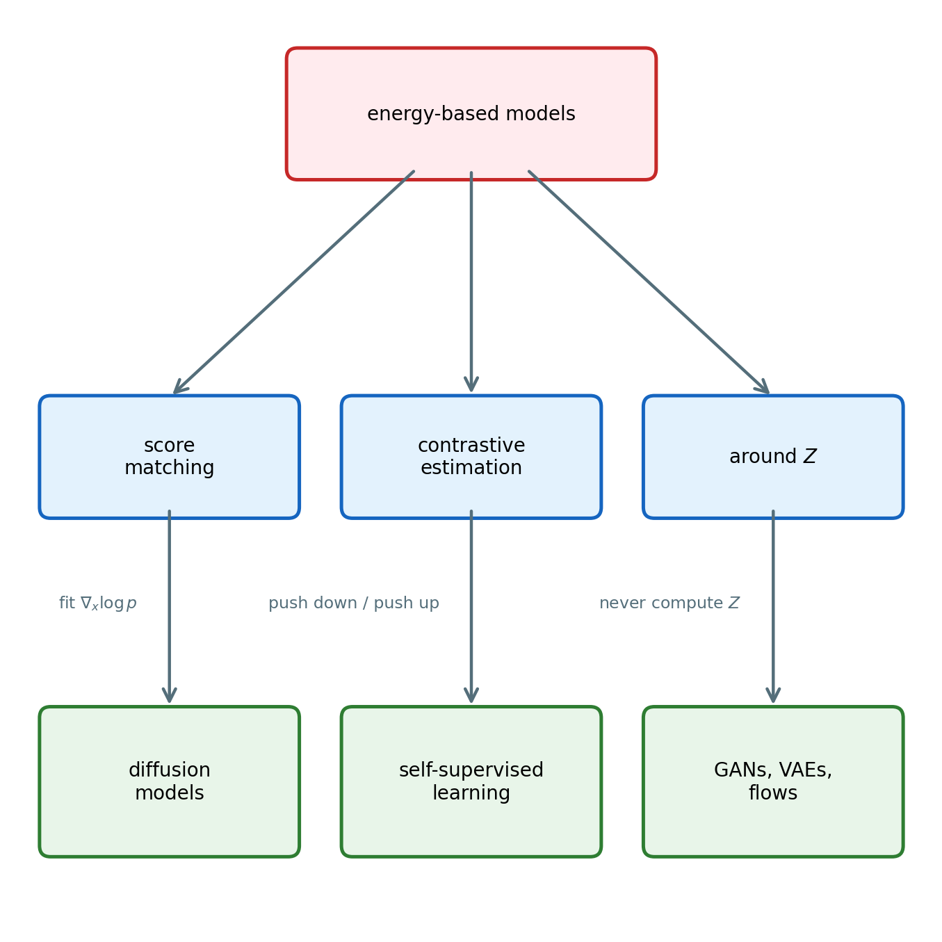
The parts that survived are the parts that never needed \(Z\).
GANs Replace the Sampler with a Generator
EBM: model \(p(\mathbf{x})\) explicitly
- Density up to \(Z\) - sampling by MCMC
- Dominant cost: the chain, every update
GAN: model the sampler directly
- A network \(G(\mathbf{z})\) = the sampler - one forward pass per sample
- No density, no \(Z\), no chain
What replaces the negative phase
- Discriminator: estimates model mass against data - a learned density ratio
- Push-up at model samples: survives, via the discriminator’s gradients
The trade
- Partition function: gone
- Sample generation: one pass
- New dominant cost: training stability
- Mode collapse replaces slow mixing
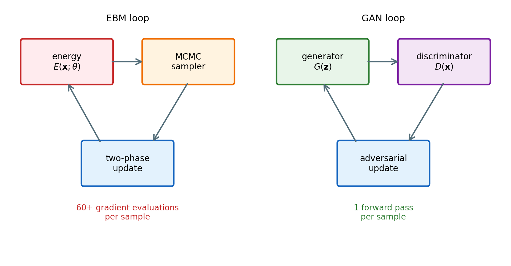
Sampling cost becomes a forward pass - the cost reappears as training instability.
GAN Samples Pass for Photographs
thispersondoesnotexist.com
- One StyleGAN2 face per reload - none of the people exist
- A family of single-model demo sites followed
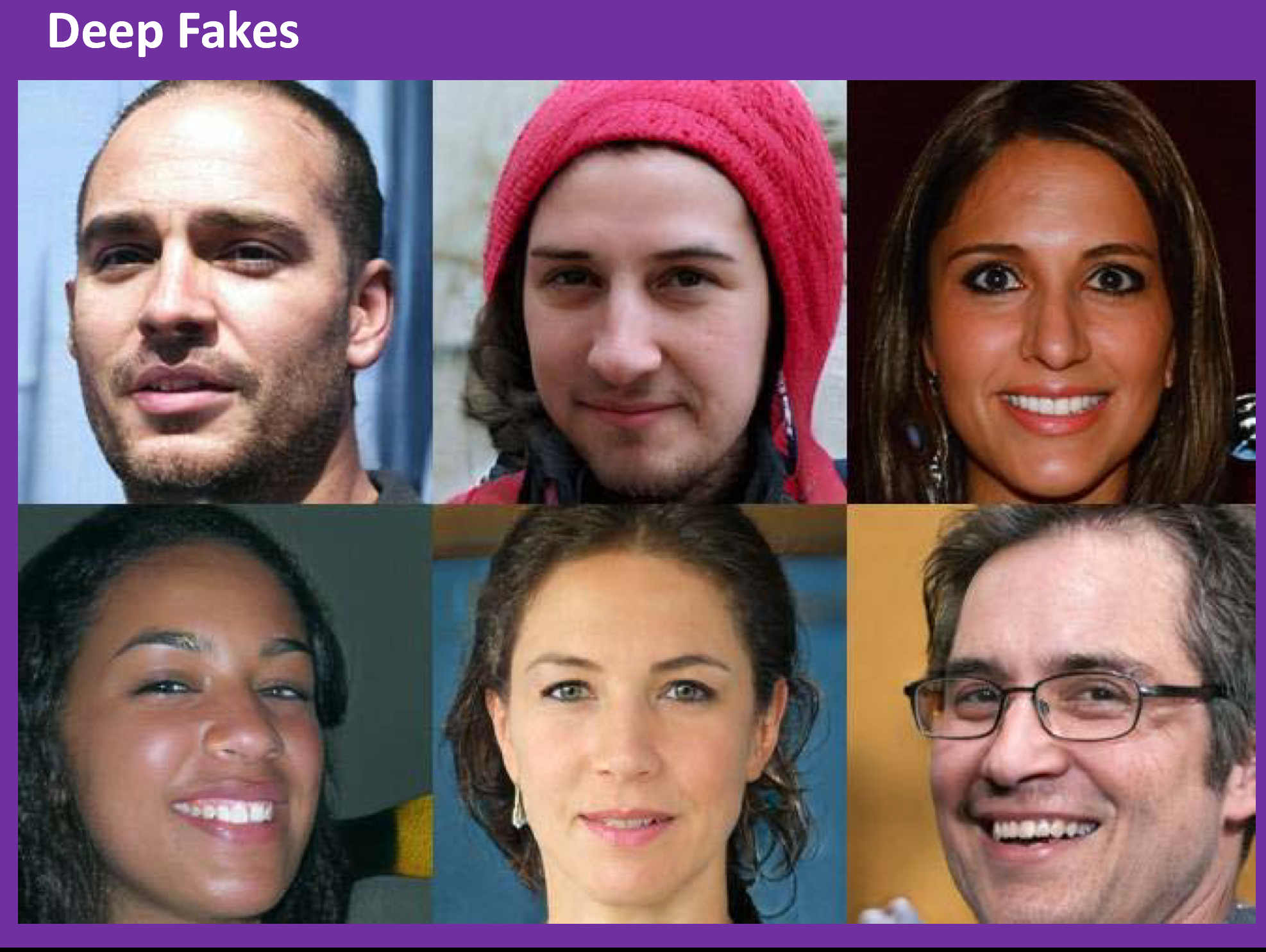
Samples: thispersondoesnotexist.com (StyleGAN2, Karras et al. 2020)
Peak numbers (FFHQ faces, 1024 × 1024)
- FID 2.84 (StyleGAN2)
- Generator: ~30M parameters
- One sample = one forward pass
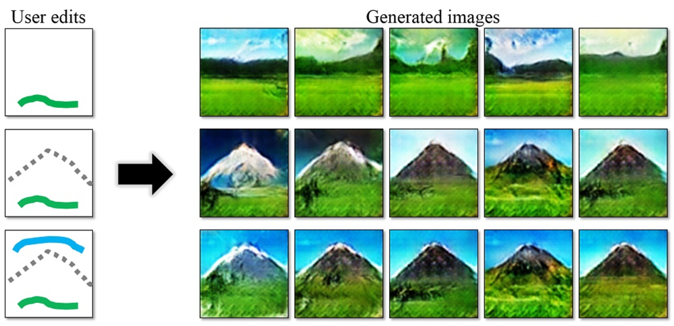
Published GAN outputs across application domains
In 2026
- Frontier image synthesis: diffusion models
- GANs persist where one fast pass matters: real-time synthesis, super-resolution, distillation targets
- Adversarial losses: still inside modern generation pipelines
Photograph-quality samples from one network pass.
GANs Began at MNIST Scale
Architecture (Goodfellow et al. 2014)
- Fully connected throughout - ReLU and sigmoid in G, maxout in D
- Predates batch norm
- Trained with the original minimax objective
Reported results
- Parzen-window log-likelihood: 225 ± 2 (MNIST)
- Parzen evaluation: itself unreliable
What was new
- Implicit generation: no Markov chains, no inference network
- Adversarial training: a learned objective in place of a likelihood
- Evolution: DCGAN → Progressive GAN → StyleGAN
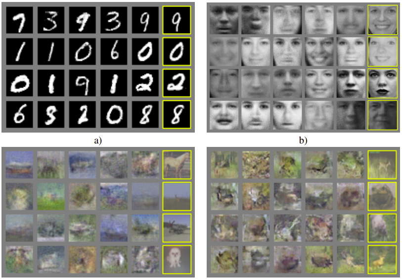
Original samples, MNIST and TFD (Goodfellow et al. 2014)
Forward and Reverse KL Penalize Opposite Errors
\[\text{KL}(p \| q) = \mathbb{E}_{x \sim p}\left[\log \frac{p(x)}{q(x)}\right]\]
Direction matters
- \(\text{KL}(p\|q) \neq \text{KL}(q\|p)\) - nonnegative, not symmetric, not a metric
Forward: \(\text{KL}(p_{\text{data}} \| q)\) - the maximum-likelihood direction
- Penalty where \(p_{\text{data}} > 0\), \(q \to 0\): unbounded - a missed mode
- Behavior: cover everything, spread thin if needed
Reverse: \(\text{KL}(q \| p_{\text{data}})\)
- Penalty where \(q > 0\), \(p_{\text{data}} \to 0\): unbounded - mass off the data
- Missing a data mode: cheap
- Behavior: concentrate on modes it keeps, drop the rest
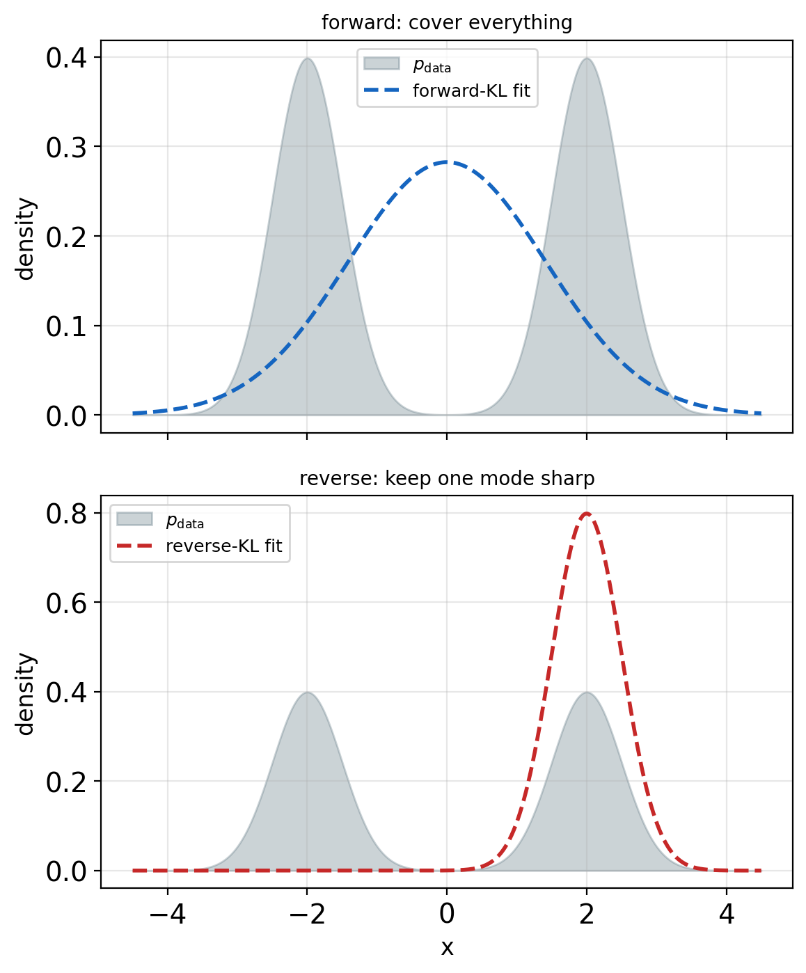
Reverse KL drops modes cheaply - the direction returns with the generator’s behavior.
A Zero-Sum Game Replaces the Likelihood
No density → no likelihood objective - training becomes a game against a learned opponent
Zero-sum game
- Two players, one value \(V\): one maximizes it, the other minimizes it
- One side’s gain = the other side’s loss
Best response
- Optimal play against a fixed opponent strategy
Minimax
- \(\min_G \max_D V(D, G)\): \(G\) optimizes against \(D\)’s best response
Nash equilibrium
- Mutual best response - neither player improves by deviating alone
- At a saddle point of \(V\): minimum along \(G\)’s directions, maximum along \(D\)’s
For GANs
- Strategies = network weights \(\boldsymbol{\theta}_G\), \(\boldsymbol{\theta}_D\) - a continuous, non-convex game
- Clean statements hold in function space - networks approximate them
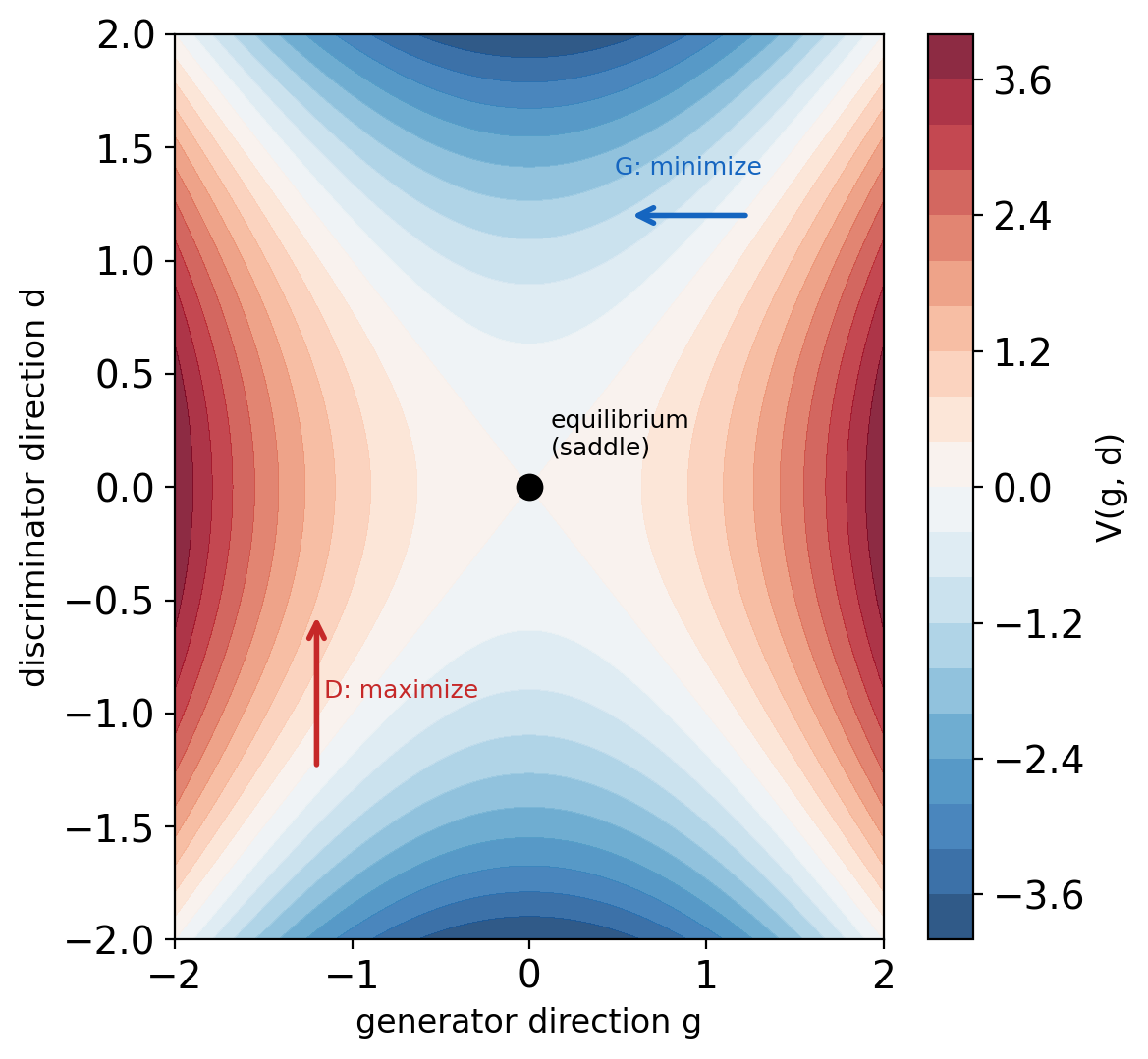
Training = seeking a saddle point, not a minimum.
The Value Function Is a Classification Loss
\[\min_G \max_D V(D,G) = \mathbb{E}_{\mathbf{x} \sim p_{\text{data}}}[\log D(\mathbf{x})] + \mathbb{E}_{\mathbf{z} \sim p(\mathbf{z})}[\log(1 - D(G(\mathbf{z})))]\]
\(D\): an ordinary binary classifier
- Class 1: real data \(\mathbf{x} \sim p_{\text{data}}\) - class 0: samples \(G(\mathbf{z})\), \(\mathbf{z} \sim p(\mathbf{z})\)
- \(D(\mathbf{x})\) = predicted probability of “real”
- \(V\) = negative binary cross-entropy - a familiar training loss, maximized
\(G\): trained through the classifier
- No direct view of the data - gradient arrives only through \(D\)
- \(\mathbf{z} \sim \mathcal{N}(0, \mathbf{I})\), samples \(G(\mathbf{z})\) - the sampler-first model from the EBM handoff
Alternation
- \(D\) step: improve the classifier at fixed \(G\)
- \(G\) step: degrade the classifier’s job at fixed \(D\)
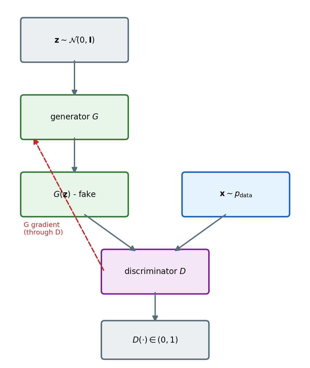
\(D\) is trained as an ordinary classifier - \(G\) is trained through it.
The Optimal Discriminator Is a Density Ratio
Fix \(G\), maximize over \(D\) pointwise
\[V(D,G) = \int_{\mathbf{x}} \left[\, p_{\text{data}}(\mathbf{x})\log D(\mathbf{x}) + p_g(\mathbf{x})\log(1 - D(\mathbf{x}))\, \right] d\mathbf{x}\]
- Per point: maximize \(f(y) = a \log y + b \log(1-y)\), with \(a = p_{\text{data}}(\mathbf{x})\), \(b = p_g(\mathbf{x})\)
\[\frac{df}{dy} = \frac{a}{y} - \frac{b}{1-y} = 0 \;\;\Rightarrow\;\; y = \frac{a}{a+b}\]
\[D^*(\mathbf{x}) = \frac{p_{\text{data}}(\mathbf{x})}{p_{\text{data}}(\mathbf{x}) + p_g(\mathbf{x})}\]
- Maximum confirmed: \(f''(y) = -a/y^2 - b/(1-y)^2 < 0\)
Reading the result
- \(D^*\) = a density-ratio estimate - likelihood information, extracted with no likelihood computed
- \(p_g = p_{\text{data}}\) → \(D^* = \tfrac{1}{2}\) everywhere: an undecidable classifier
- The contrastive push-down/push-up idea, as a classifier
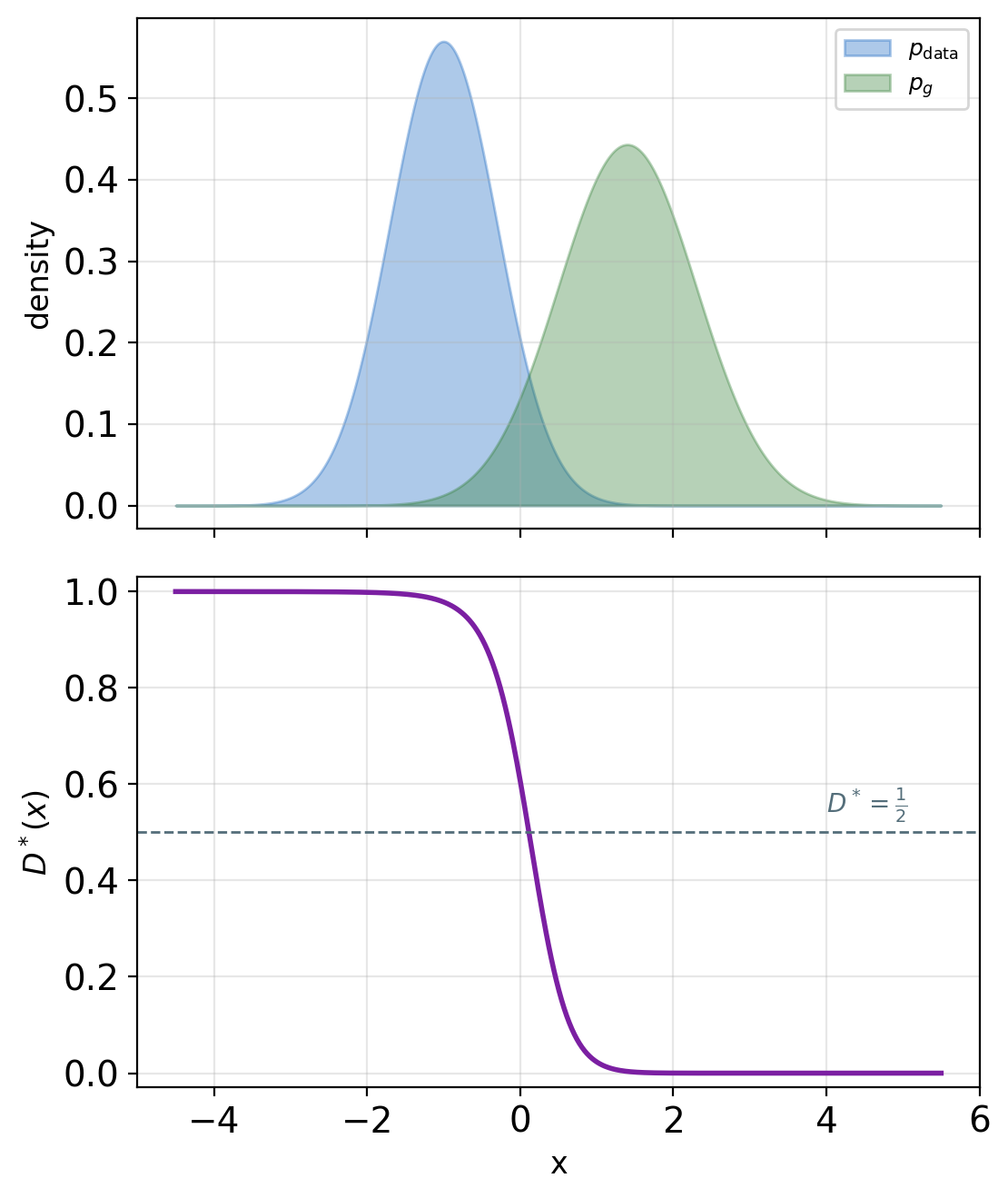
The optimal classifier’s confidence encodes where the two distributions disagree.
At Optimal D the Generator Minimizes JS
Substitute \(D^*\) into the value
\[C(G) = \mathbb{E}_{p_{\text{data}}}\!\left[\log \frac{p_{\text{data}}}{p_{\text{data}} + p_g}\right] + \mathbb{E}_{p_g}\!\left[\log \frac{p_g}{p_{\text{data}} + p_g}\right]\]
\[C(G) = -\log 4 + 2\, \text{JS}(p_{\text{data}} \| p_g)\]
Jensen-Shannon divergence
\[\text{JS}(p \| q) = \tfrac{1}{2}\text{KL}(p \| m) + \tfrac{1}{2}\text{KL}(q \| m), \qquad m = \tfrac{1}{2}(p + q)\]
- Symmetric, and \(0 \leq \text{JS} \leq \log 2\)
- Zero iff \(p = q\) - the minimax optimum is exactly \(p_g = p_{\text{data}}\)
- \(\log 2\) = the ceiling, reached when \(p\) and \(q\) share no mass
Saturation
- Two distributions that barely overlap: JS pinned near \(\log 2\), nearly flat in \(p_g\)
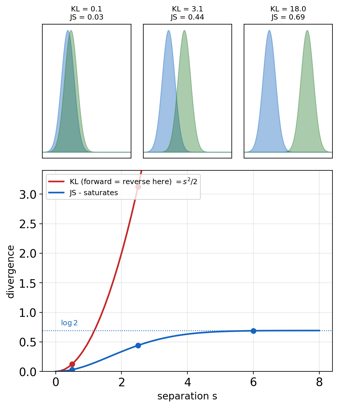
With a perfect critic, adversarial training is JS minimization.
Each KL Penalizes a Different Failure
With separated modes, each KL reduces to a KL between the mixture weights
Removing a data mode - \(p_{\boldsymbol{\theta}}\)’s weight on one data mode \(\to 0\)
- Forward KL: grows without bound
- Reverse KL: \(\to \log 2\) - the weight cost \(\mathrm{KL}\!\left((1{-}w, w) \,\|\, (\tfrac{1}{2}, \tfrac{1}{2})\right)\) alone - zero from the missing region
- JS: \(\to 0.22\) - bounded
Adding a spurious mode - \(p_{\boldsymbol{\theta}}\) mass where \(p_{\text{data}}\) has none
- Reverse KL: explodes
- Forward KL: \(-\log(1 - v)\) - the true mode’s dilution alone - zero from the spurious region
- JS: bounded again
Objective vs behavior
- JS is the objective at optimal \(D\)
- The generator’s loss in use determines which divergence training follows
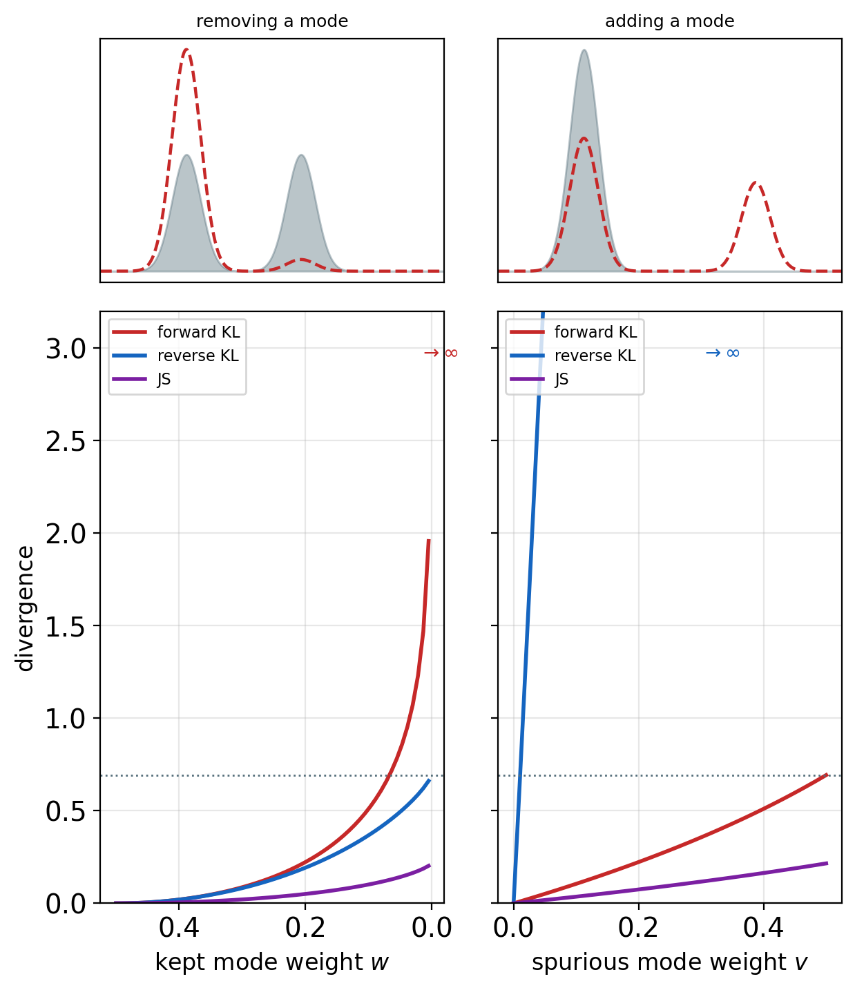
Forward KL penalizes missing modes, reverse KL penalizes spurious mass - JS bounds both.
Discriminator Saturation Cuts the Generator’s Gradient
Early training: \(G\) poor → \(D\) separates easily → \(D(G(\mathbf{z})) \to 0\)
Differentiate in logit space - \(D = \sigma(a)\), gradients reach \(G\) through \(a\)
- Saturating loss (the minimax original):
\[\frac{\partial}{\partial a} \log(1 - \sigma(a)) = -\sigma(a) = -D\]
- Non-saturating alternative, \(\max_G \log D\):
\[\frac{\partial}{\partial a} \log \sigma(a) = 1 - \sigma(a) = 1 - D\]
Same fixed points, opposite failure
- \(D(G(\mathbf{z})) \approx 0\): saturating gradient \(\approx 0\) - non-saturating \(\approx 1\)
- The loss-level view of the JS plateau: barely-overlapping distributions, flat objective
- Non-saturating: standard practice
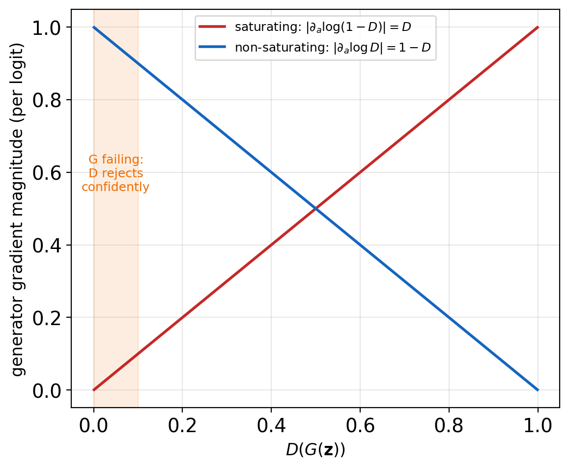
Under the saturating loss, the gradient to \(G\) is weakest exactly when \(G\) is worst.
Collapse Is Optimal Under the Effective Objective
Reverse KL, applied
- Spurious mass off the data: unbounded penalty - stay on modes
- A dropped mode: \(\log(1/w)\) nats - affordable
- Limited capacity → match a subset of modes exactly
Two named failures
- Mode dropping: a subset of modes missing, the rest sharp
- Mode collapse: outputs concentrate on one mode or point
The cycle in practice
- \(G\) concentrates on one mode
- \(D\) learns to reject that region
- \(G\) jumps to another mode
- Repeat - oscillation, not convergence
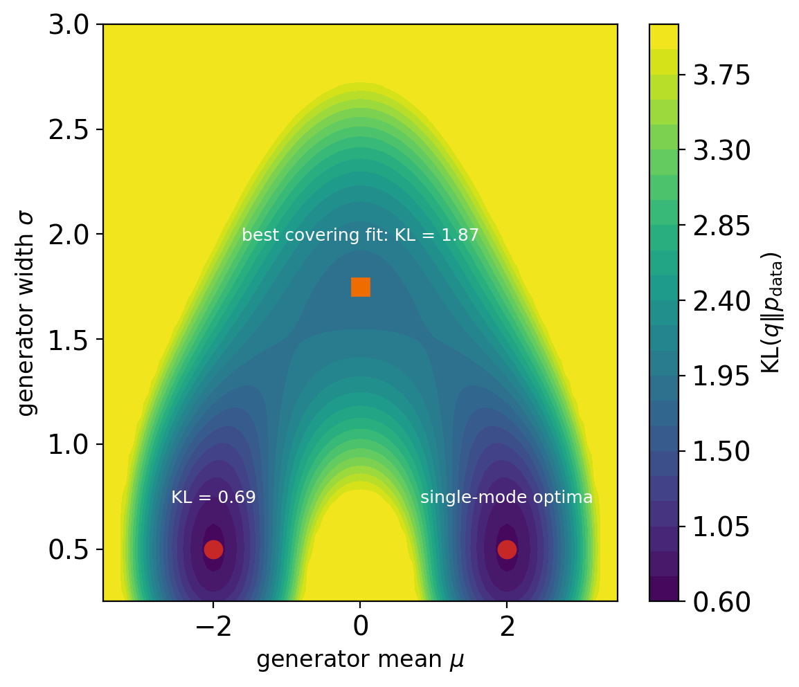
Collapse follows the objective - not an optimizer failure.
Simultaneous Gradient Updates Can Orbit Forever
Equilibrium exists - in function space
- \(p_g = p_{\text{data}}\), \(D = \tfrac{1}{2}\) everywhere: a Nash point of the game
- Convergence proof (Goodfellow et al. 2014): convexity in function space, \(D\) optimal at every step
- Networks train in parameter space - non-convex, \(D\) never optimal
Simultaneous updates on the simplest saddle - \(V(g, d) = g \cdot d\)
- \(G\) descends, \(D\) ascends, simultaneously: \(\dot{g} = -d\), \(\;\dot{d} = g\)
- Continuous time: circles around the equilibrium - never approaching it
- Discrete steps: each update multiplies the radius by \(\sqrt{1 + \eta^2}\) - an outward spiral
Observed GAN training
- Losses oscillate - no reliable stopping signal in the loss values
- Stopping: sample-quality metrics, not loss
- Averaged generator weights (EMA): smooths the orbit’s iterates
Update ratios
- \(D\) steps per \(G\) step: a design choice - more \(D\) steps → closer to the optimal-\(D\) assumption
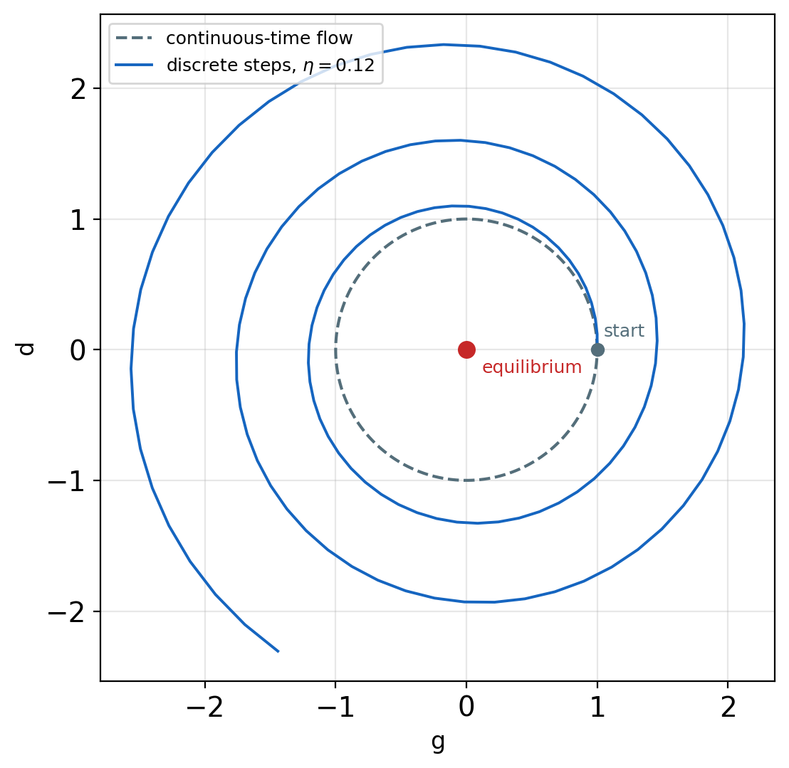
The saddle exists - simultaneous gradient updates do not converge to it by default.
Label Smoothing Works One-Sided Only
Targets (Salimans et al. 2016)
- Real side softened → D stops at 0.9 confidence - weaker saturating pressure
Why the fake side stays at zero
- Smoothed targets \(\alpha\) (real), \(\beta\) (fake) → optimal discriminator:
\[D^*(\mathbf{x}) = \frac{\alpha\, p_{\text{data}}(\mathbf{x}) + \beta\, p_g(\mathbf{x})}{p_{\text{data}}(\mathbf{x}) + p_g(\mathbf{x})}\]
- \(\beta > 0\): where \(p_g \gg p_{\text{data}}\), \(D^* \approx \beta\) - spurious samples keep a nonzero score
- \(G\)’s current mistakes get rewarded exactly where they live
- \(\beta = 0\): spurious regions still driven to zero
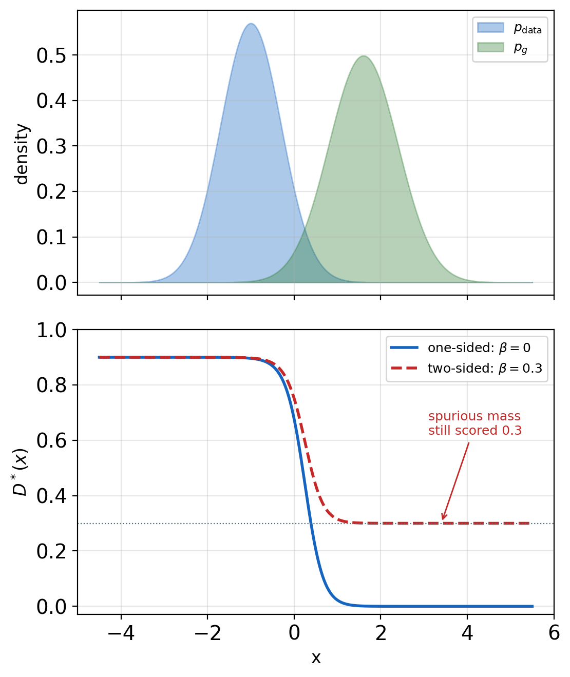
Fake-side smoothing rewards exactly the samples training should reject.
Spectral Normalization Caps the Discriminator’s Slope
One line per layer (Miyato et al. 2018)
\[\mathbf{W}_{\text{SN}} = \frac{\mathbf{W}}{\sigma(\mathbf{W})}, \qquad \sigma(\mathbf{W}) = \text{largest singular value}\]
- \(\sigma\) by one power-iteration step per update - negligible cost
- Every layer 1-Lipschitz + 1-Lipschitz activations → a network-wide slope cap
Placement
- All \(D\) layers (Miyato et al. 2018)
- \(G\) too, at scale (BigGAN)
Measured (CIFAR-10 unconditional, Inception Score)
- Weight clipping 6.41 → WGAN-GP 6.68 → layer norm 7.19 → spectral norm 7.42
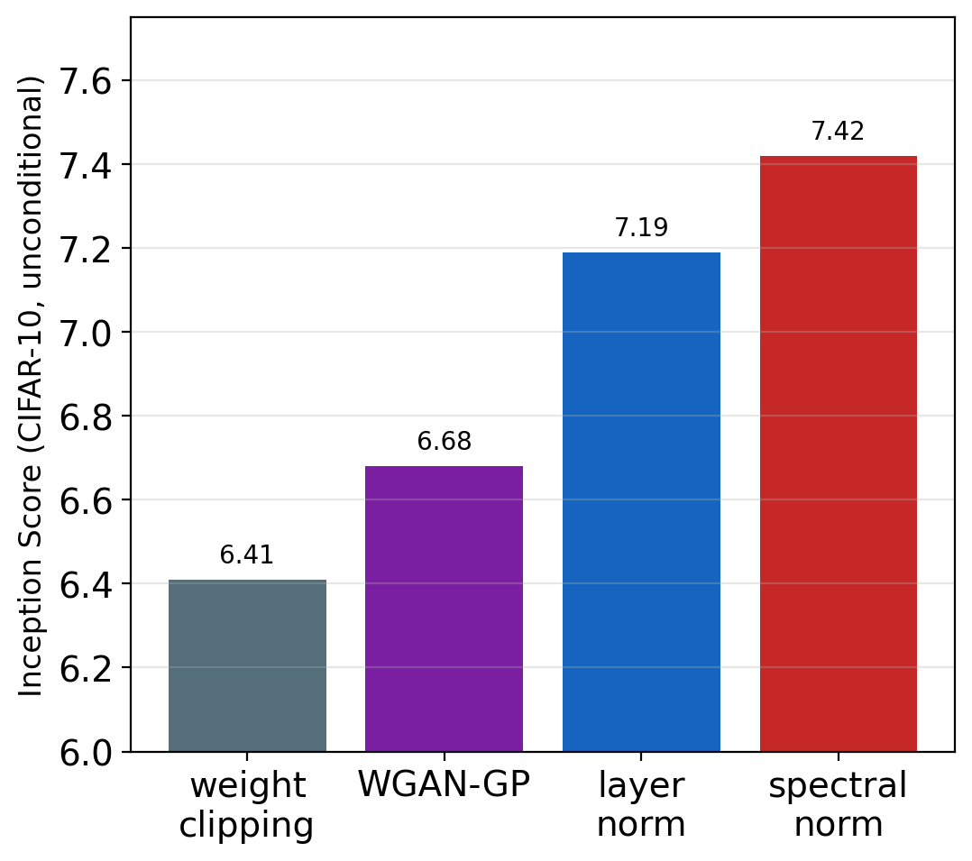
Why a slope cap is the right constraint: the Wasserstein distance supplies the reason.
Real Data Lives on Thin Sets
Support - where a distribution puts its mass
Image data is thin in pixel space
- Pixel space: \(d \sim 10^5\) dimensions - valid images: a vanishing, structured subset
- Locally few directions of variation (pose, lighting, identity) - a low-dimensional manifold, embedded in \(\mathbb{R}^d\)
Generated data is thin by construction
- \(p_g\) = the image of \(\mathbf{z} \in \mathbb{R}^{100}\) under \(G\) - dimension ≤ 100, whatever \(G\) does
Two thin sets rarely meet (Arjovsky and Bottou 2017)
- Low-dimensional sets in high dimension: generically zero shared mass
- Disjoint supports → a perfect discriminator exists at every step
- JS pinned at \(\log 2\) → the saturation plateau is the generic case, not early-training bad luck
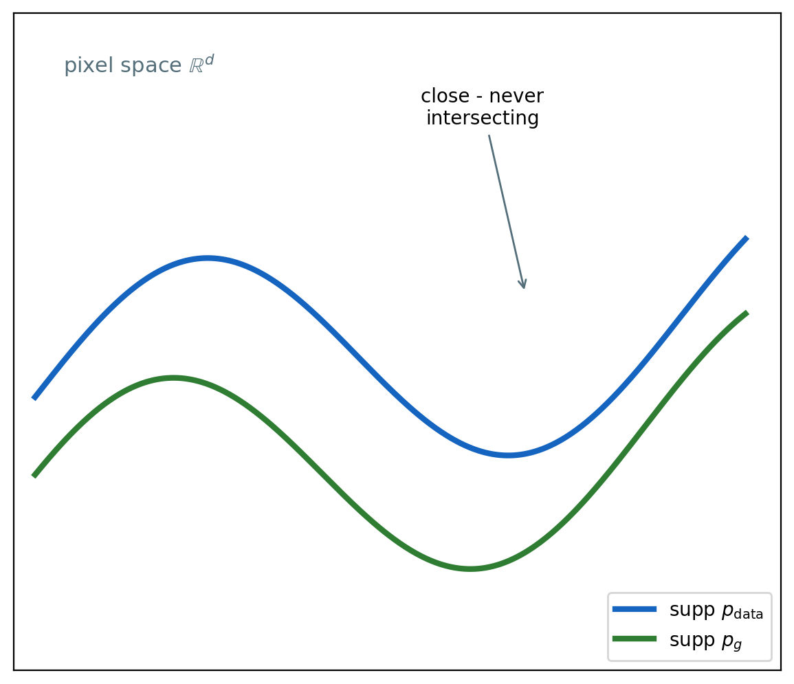
The JS plateau is generic for image models - the objective needs replacing, not the optimizer.
Earth Mover’s Distance Measures Transport
\[W(p, q) = \inf_{\gamma \in \Pi(p, q)} \; \mathbb{E}_{(\mathbf{x}, \mathbf{y}) \sim \gamma}\left[\, \|\mathbf{x} - \mathbf{y}\|\, \right]\]
Reading the definition
- \(\Pi(p, q)\): joint distributions with marginals \(p\) and \(q\) - the transport plans
- \(\gamma(\mathbf{x}, \mathbf{y})\): how much mass moves from \(\mathbf{x}\) to \(\mathbf{y}\)
- \(W\) = cheapest total mass × distance - defined with or without overlap
Two point masses, separation \(\alpha\)
- \(\text{JS}(\delta_0 \| \delta_\alpha) = \log 2\) for every \(\alpha \neq 0\) - blind to how far
- \(W(\delta_0, \delta_\alpha) = \alpha\) - the distance itself
What that buys the generator - a slope toward the data even from far away
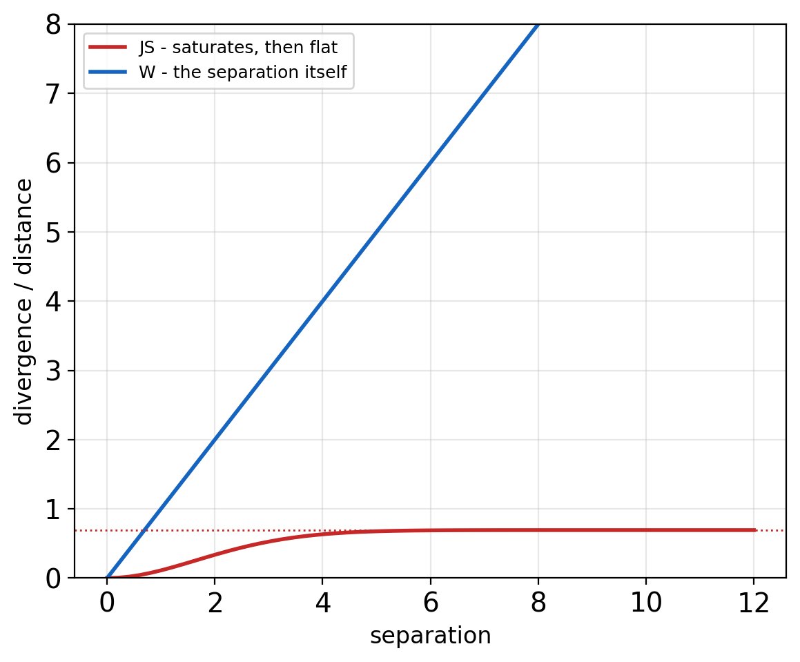
W varies smoothly with separation - JS stops at \(\log 2\).
Duality Turns Transport into a Critic
Kantorovich-Rubinstein duality
\[W(p, q) = \sup_{\|f\|_L \leq 1} \; \mathbb{E}_{\mathbf{x} \sim p}[f(\mathbf{x})] - \mathbb{E}_{\mathbf{y} \sim q}[f(\mathbf{y})]\]
Lipschitz constraint - \(\|f\|_L \leq 1\):
\[|f(\mathbf{x}_1) - f(\mathbf{x}_2)| \leq \|\mathbf{x}_1 - \mathbf{x}_2\|\]
- Slope bounded by 1, everywhere
What duality changes
- Primal: optimize over transport plans \(\gamma\) - intractable
- Dual: optimize over functions \(f\) - a neural network’s job
- \(f\) = the critic: real-valued scores, not probabilities
Why the cap is essential
- Unconstrained \(f\): send \(f \to +\infty\) on \(p\), \(-\infty\) on \(q\) - supremum diverges
- The bound ties the score difference to actual distance
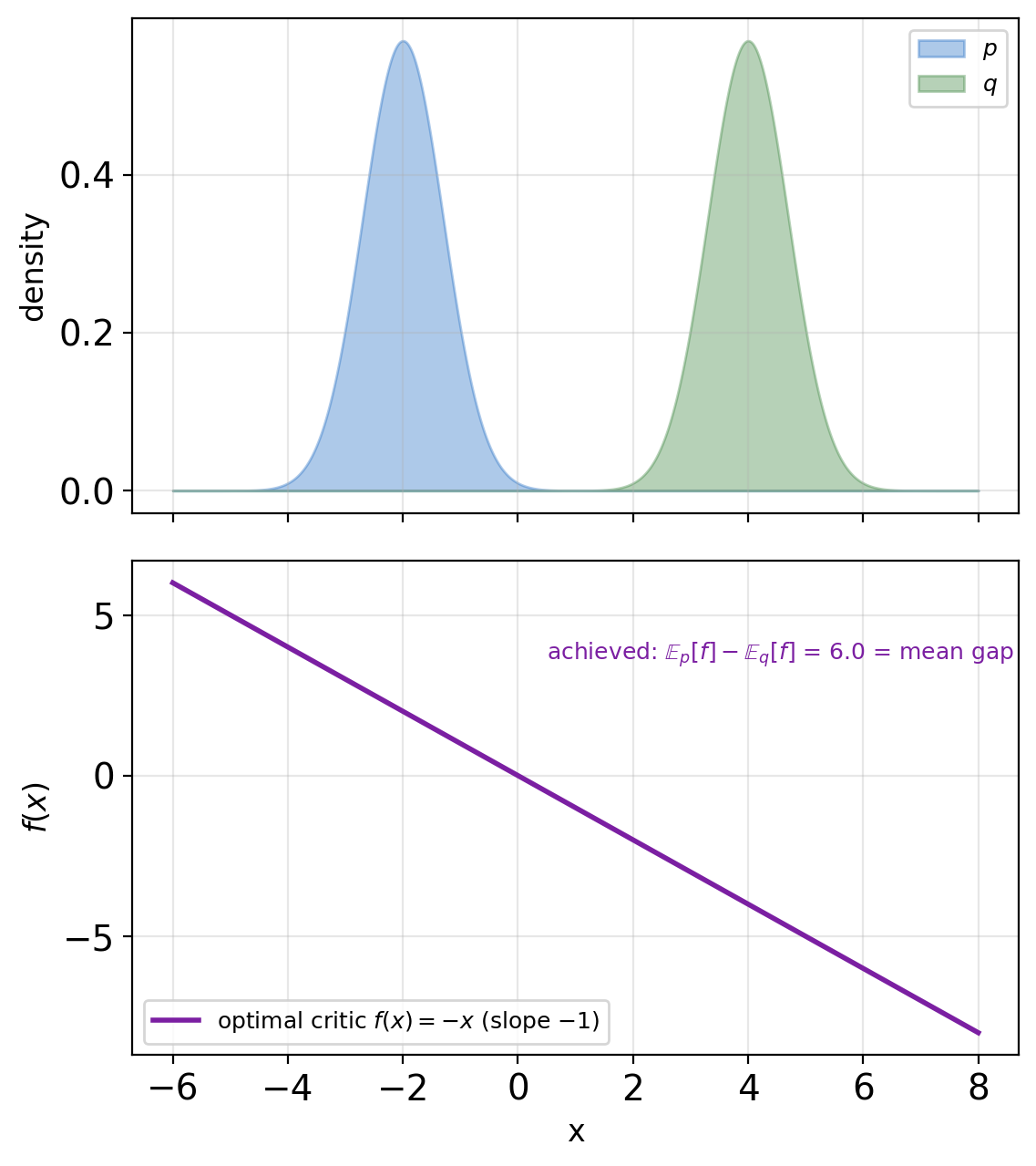
Remove the slope cap and the supremum diverges - the constraint is the metric.