Generative Models: GAN Architectures, Evaluation, and VAEs
EE 641 - Unit 3B
Transposed Convolution Upsamples Inside the Network
Shapes
- Convolution, stride 1: \(H \times W \to H \times W\)
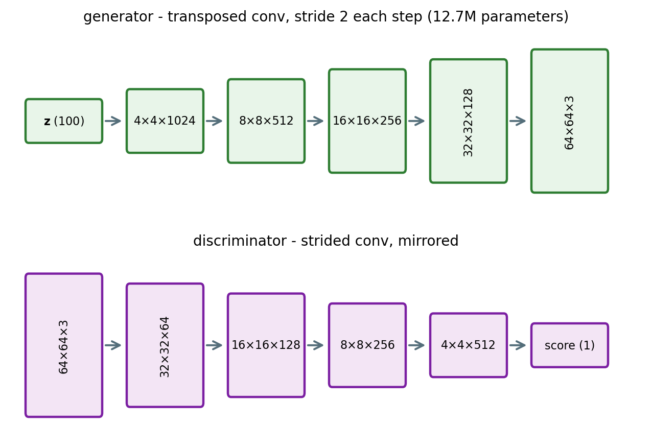
- Transposed, stride 2: \(H \times W \to 2H \times 2W\) - upsampling as a learned layer
- Parameters both ways: \(K^2 \cdot C_{\text{in}} \cdot C_{\text{out}}\)
- Equivalent form: insert a zero between neighboring inputs, then convolve - the transpose’s sparsity pattern made explicit
Matrix reading
- Convolution: \(\mathbf{y} = \mathbf{W}\mathbf{x}\), \(\mathbf{W}\) sparse
- Transposed: \(\mathbf{y} = \mathbf{W}^\top \mathbf{x}\) - the transpose, not the inverse: \(\mathbf{W}^\top \mathbf{W} \neq \mathbf{I}\)
Checkerboard artifacts
- Kernel size not divisible by stride: uneven overlap in the output
- Fixes: stride = kernel size, or resize then convolve
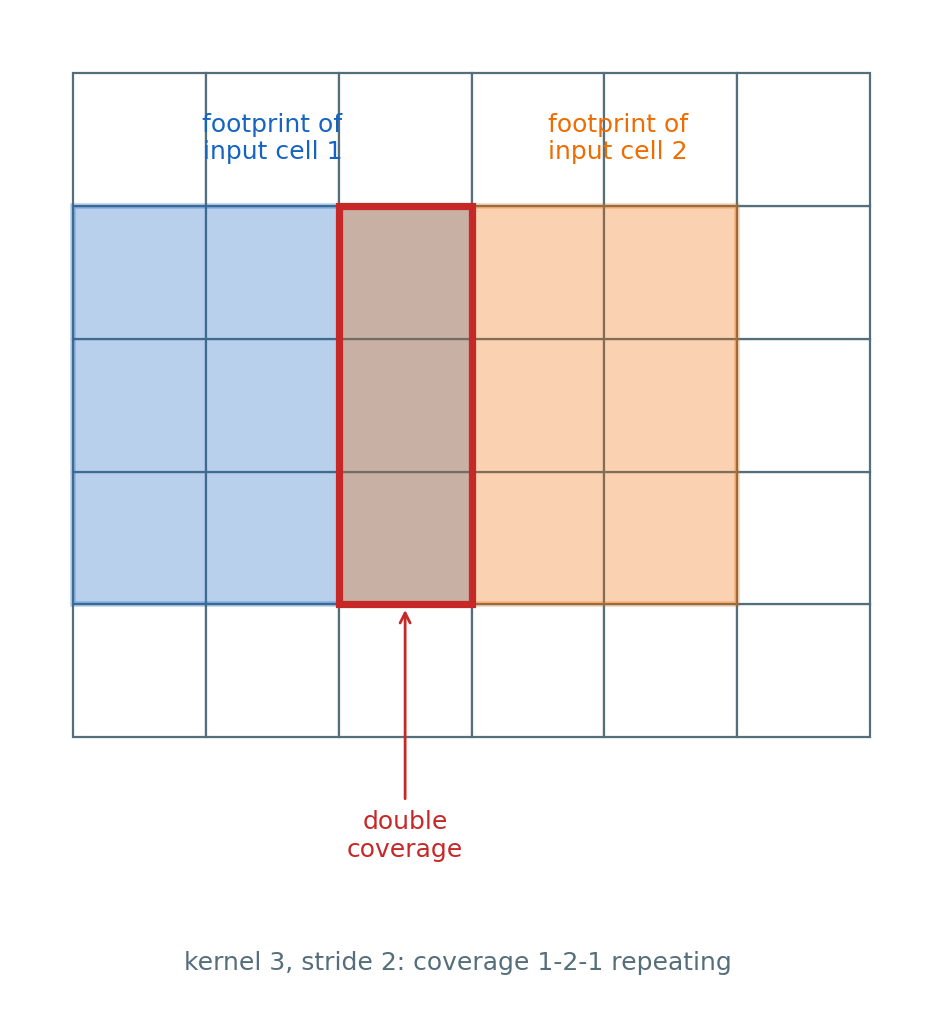
Resize-then-convolve removes the overlap pattern by giving up the learned upsampling - the trade behind the checkerboard fix.
Four Rules Stabilized Convolutional GAN Training
Four architecture rules (Radford et al. 2016)
- All-convolutional: strided convolutions replace pooling, no fully connected hidden layers
- Batch norm: every \(G\) layer except the output, every \(D\) layer except the input
- Activations: ReLU in \(G\) with tanh output - LeakyReLU (0.2) throughout \(D\)
- Upsampling: transposed convolutions, stride 2 per resolution doubling
What changed
- Training that succeeds across datasets (LSUN bedrooms, faces, ImageNet) without per-dataset tuning
- Vector arithmetic in \(\mathbf{z}\) - directions with meaning
Size
- Generator ≈ 12.7M parameters - two thirds in the first transposed convolution (\(4 \cdot 4 \cdot 1024 \cdot 512\))
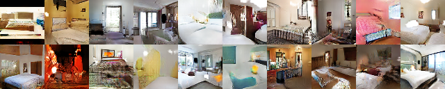
LSUN bedrooms, 64 × 64, after five epochs (Radford et al. 2016, Fig. 3)
Later generators keep this stride-2 pyramid and change what feeds it - the schedule, the code, the normalization.
Conditioning Adds Control at Both Networks
\[\min_G \max_D\; \mathbb{E}_{\mathbf{x}, y}\!\left[\log D(\mathbf{x} | y)\right] + \mathbb{E}_{\mathbf{z}, y}\!\left[\log(1 - D(G(\mathbf{z} | y) | y))\right]\]
Both networks see the condition (Mirza and Osindero 2014)
- \(G(\mathbf{z}, y)\): generate for a given \(y\) - \(D(\mathbf{x}, y)\): judge the pair
- \(y\): class label, text embedding, another image - any side information
Failure it introduces
- Within-class collapse: \(G(\cdot, y)\) returns one image per \(y\) - varied across classes, confident, and invisible to a class-based score
Three injection routes
- Concatenation: \(y\) appended to the input - the original form
- Projection (Miyato and Koyama 2018): an inner product between features and a class embedding - used by SAGAN and BigGAN
- AdaIN: normalize each sample’s channels, then scale and shift by a function of \(y\) - the route StyleGAN builds on
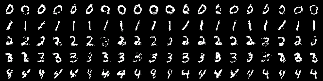
One row per label \(y\) (0 to 4 shown), \(\mathbf{z}\) varying along the row (Mirza and Osindero 2014, Fig. 2)
All three routes leave the objective unchanged - the condition changes what \(G\) and \(D\) compute, not what they optimize.
Conditioning Splits \(D^*\) into Two Log-Ratios
From the density ratio - on pairs \((\mathbf{x}, y)\), \(D^* = p/(p+q)\) and its logit is a log-ratio:
\[a^*(\mathbf{x}, y) = \log \frac{p(\mathbf{x}, y)}{q(\mathbf{x}, y)} = \underbrace{\log \frac{p(y|\mathbf{x})}{q(y|\mathbf{x})}}_{\text{class term}} + \underbrace{\log \frac{p(\mathbf{x})}{q(\mathbf{x})}}_{\text{unconditional}}\]
- Unconditional term: the ordinary discriminator on \(\mathbf{x}\) alone - a network \(\psi(\phi(\mathbf{x}))\)
- Class term: how the two class-posteriors disagree at \(\mathbf{x}\) - the only place \(y\) enters
Log-linear class model
- Assumption: \(p(y|\mathbf{x}) \propto \exp(\mathbf{v}_y^{p\top} \phi(\mathbf{x}))\), and likewise for \(q\) - both class-posteriors are softmax classifiers on shared features
- Class term \(= (\mathbf{v}^p_y - \mathbf{v}^q_y)^\top \phi(\mathbf{x})\) plus terms independent of \(y\)
- Collected: \(a^*(\mathbf{x}, y) = \mathbf{y}^\top \mathbf{V}\, \phi(\mathbf{x}) + \psi(\phi(\mathbf{x}))\) - the projection discriminator (Miyato and Koyama 2018)
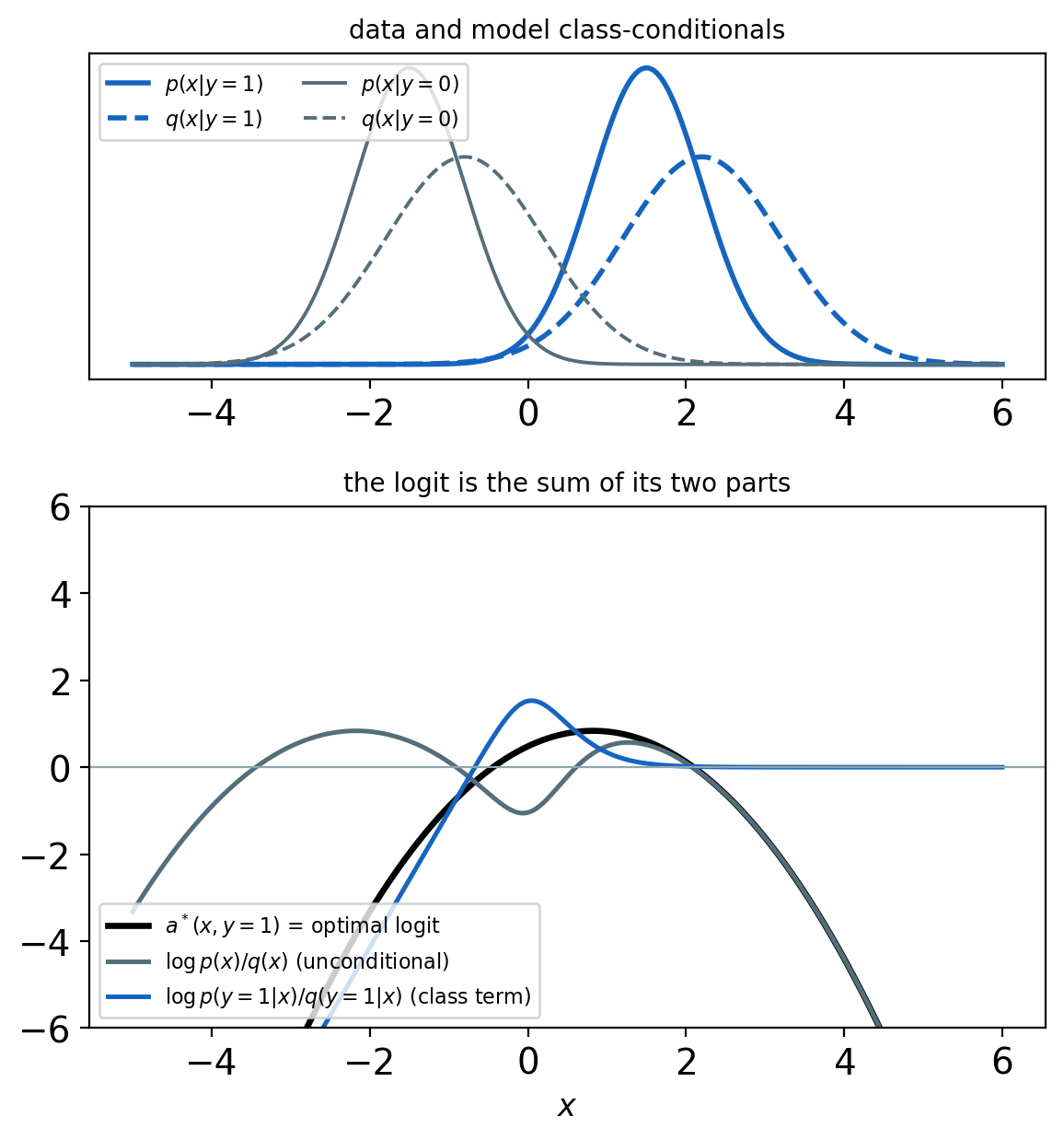
Projection hard-codes the additive class term - concatenation has to learn it.
Progressive Growing Stabilizes High Resolution
Schedule (Karras et al. 2018)
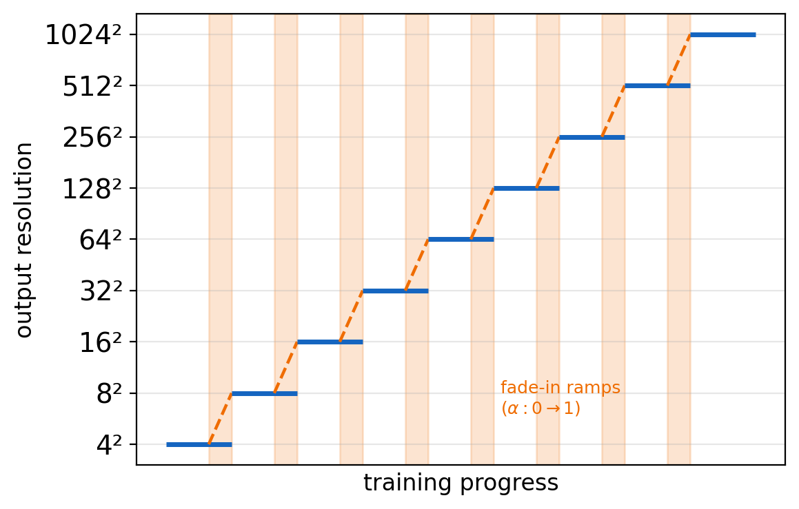
- Train at 4 × 4 for a fixed image budget - add a resolution-doubling block - repeat to 1024 × 1024
- Every added block fades in: \(\alpha\) from 0 to 1
What the schedule changes
- Low-resolution stages settle layout - later stages add detail only
- Why it stabilizes: each new stage starts from a generator that already matches the coarse statistics - the supports overlap, and the discriminator has no free win
- Up to 5.4× faster to a fixed quality at 1024² (Karras et al. 2018)
- First 1024 × 1024 face samples (CelebA-HQ)
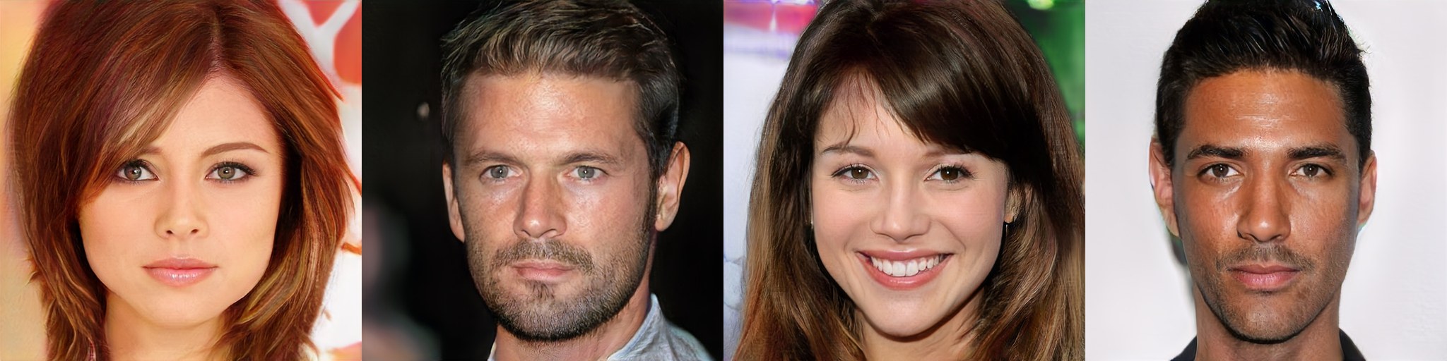
CelebA-HQ samples at 1024 × 1024 (Karras et al. 2018, Fig. 5)
The high-resolution game never starts from scratch - it inherits the overlap the low-resolution stage established.
StyleGAN Injects One Code at Every Scale
Three changes to the generator (Karras et al. 2019)
- Mapping network: \(\mathbf{z} \to \mathbf{w}\) through 8 FC layers - \(\mathbf{w}\)-space less entangled than \(\mathbf{z}\)-space, measured by perceptual path length and linear separability
- Style injection: \(\mathbf{w}\) enters every synthesis block through AdaIN - coarse blocks set pose and shape, fine blocks set color and texture
- Per-layer noise: fresh randomness at each scale - stochastic detail (hair, freckles) without structural change
Lineage and cost
- StyleGAN2: weight demodulation replaces AdaIN - removes the blob artifacts of per-sample normalization - and path-length regularization added
- StyleGAN3: alias-free synthesis - texture no longer locked to pixel coordinates
- StyleGAN2 at FFHQ 1024²: ~30M generator parameters, ~9 days on 8 V100s (Karras et al. 2020)
- FID on FFHQ 1024², one dataset across the lineage: 8.04 (Progressive GAN), 4.40 (StyleGAN), 2.84 (StyleGAN2)
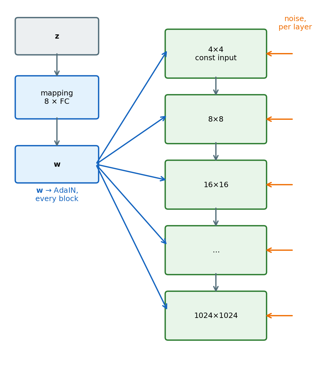
Because every block receives \(\mathbf{w}\) separately, a code can be swapped per band - the basis of style mixing and of truncation in \(\mathbf{w}\).
Coarse Styles Set Pose, Fine Styles Set Color
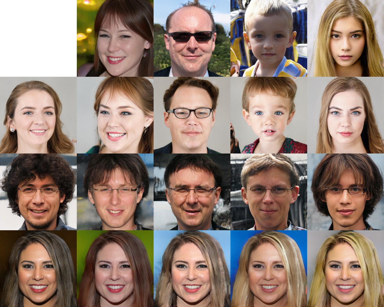
Style mixing on FFHQ (Karras et al. 2019, Fig. 3; tiles from the paper’s source)
Two latent codes, one image
- Top row: source A, four samples - left column: source B, three samples
- Each interior image: \(\mathbf{w}_B\) everywhere, with \(\mathbf{w}_A\) substituted in one band of blocks
What each band carries
- Row 1, coarse blocks (\(4^2\) to \(8^2\)) from A: pose, face shape, glasses, hair style follow A - colors stay B’s
- Row 2, middle blocks (\(16^2\) to \(32^2\)) from A: facial features and eyes follow A - pose stays B’s
- Row 3, fine blocks (\(64^2\) to \(1024^2\)) from A: color scheme and micro-texture follow A - identity stays B’s
Read against the synthesis stack
- The band a style is applied to is the scale it controls - the synthesis stack’s routing, read off the images
Attributes separate by scale because the code is applied by scale.
Latent Interpolation Stays on the Manifold
Paths in \(\mathbf{z}\) decode to paths on the manifold
- Interpolate in \(\mathbf{z}\) (or \(\mathbf{w}\)): \(G\) is continuous, so the decoded path stays on the output manifold - a smooth morph
- Straight lines in a Gaussian \(\mathbf{z}\) cut through the low-mass interior - spherical interpolation keeps the path on the typical shell \(\|\mathbf{z}\| \approx \sqrt{d}\) (White 2016)
- Interpolate in pixel space: the straight line leaves the data manifold - cross-fades, not intermediates
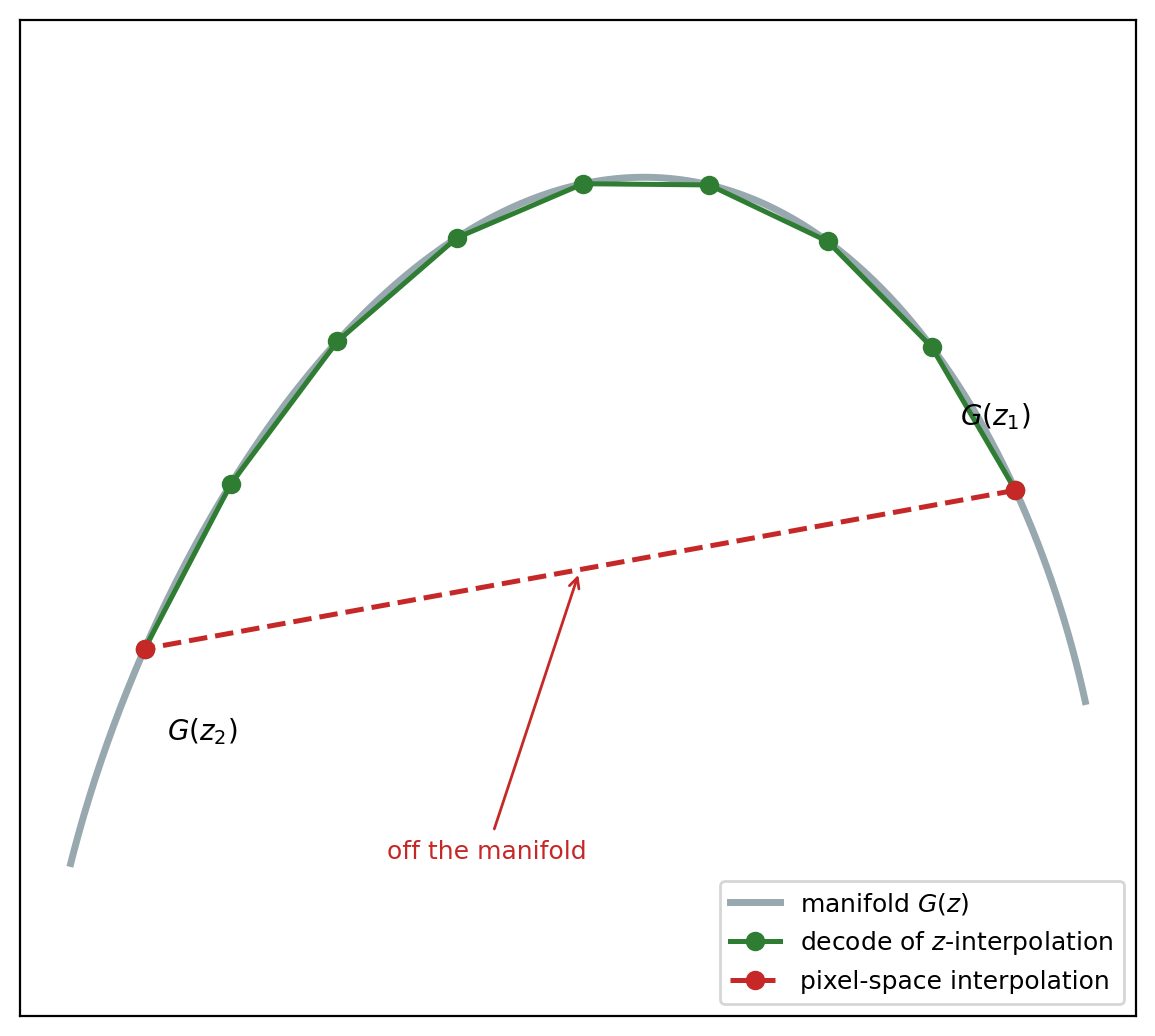
Interpolation is the standard check that \(G\) generalizes - a memorizing \(G\) would cross-fade between training images.
Latent Arithmetic Works Where Pixel Arithmetic Fails
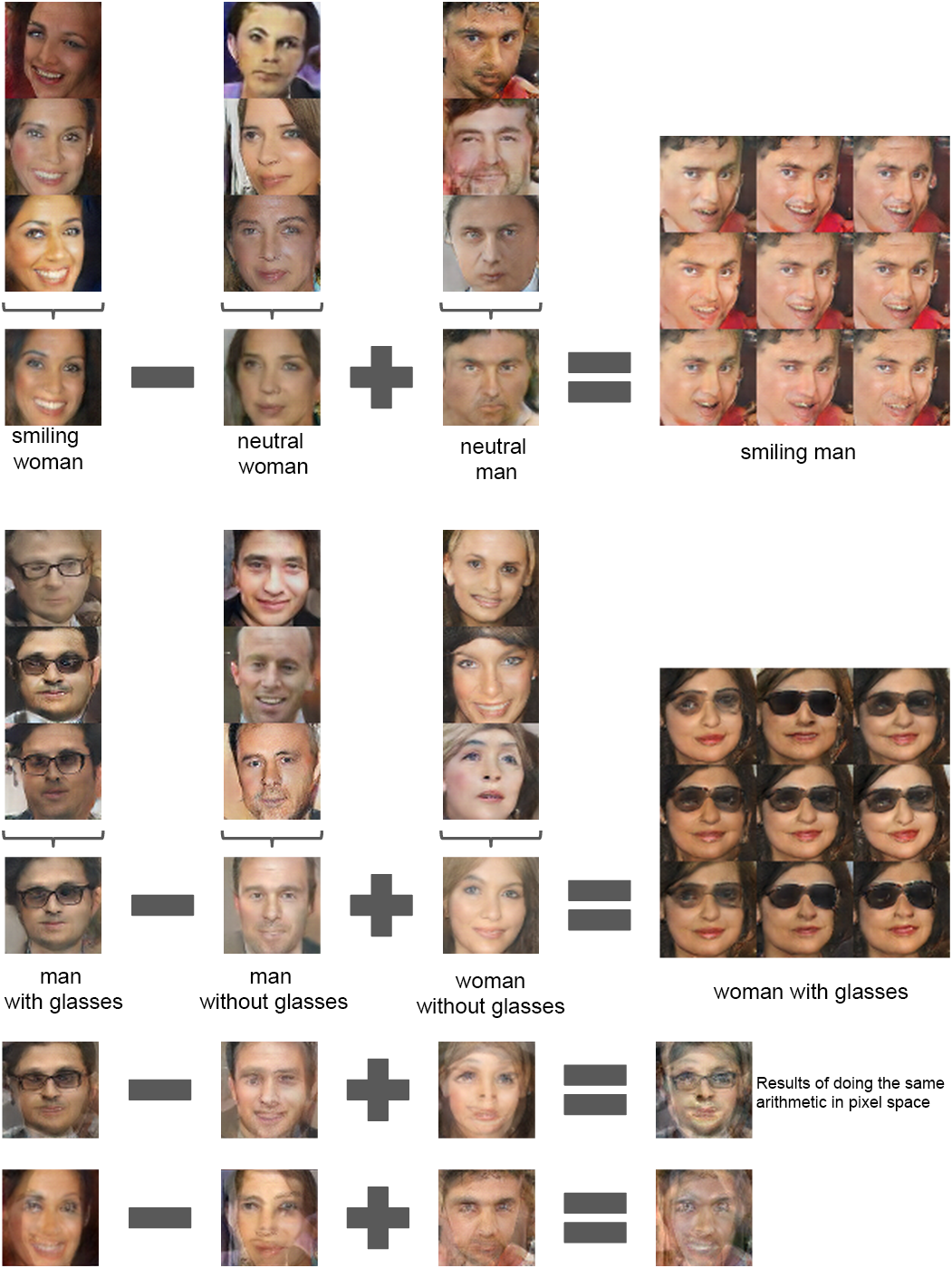
DCGAN on faces (Radford et al. 2016, Fig. 7)
Procedure (Radford et al. 2016)
- Average the \(\mathbf{z}\) of three samples sharing an attribute - one vector per concept
- \(\mathbf{z}_{\text{smiling woman}} - \mathbf{z}_{\text{neutral woman}} + \mathbf{z}_{\text{neutral man}}\), decoded: a smiling man
- The \(3 \times 3\) block: the result plus small perturbations of \(\mathbf{z}\) - the direction is stable under them
Averaging
- One sample’s \(\mathbf{z}\) carries everything about that face - averaging three cancels what they do not share
Same arithmetic in pixel space (bottom rows)
- Averaged faces blur, differences of averages ghost - no pixel-space direction corresponds to smiling
What it shows
- Linear attribute directions in \(\mathbf{z}\) are observed, not guaranteed - nothing in the objective asks for them, and they appear when attributes vary independently in the data
Arithmetic in \(\mathbf{z}\) works when attributes occupy separable directions - a property \(G\) acquired, not one the objective imposed.
Truncation Trades Diversity for Fidelity in \(\mathbf{w}\)
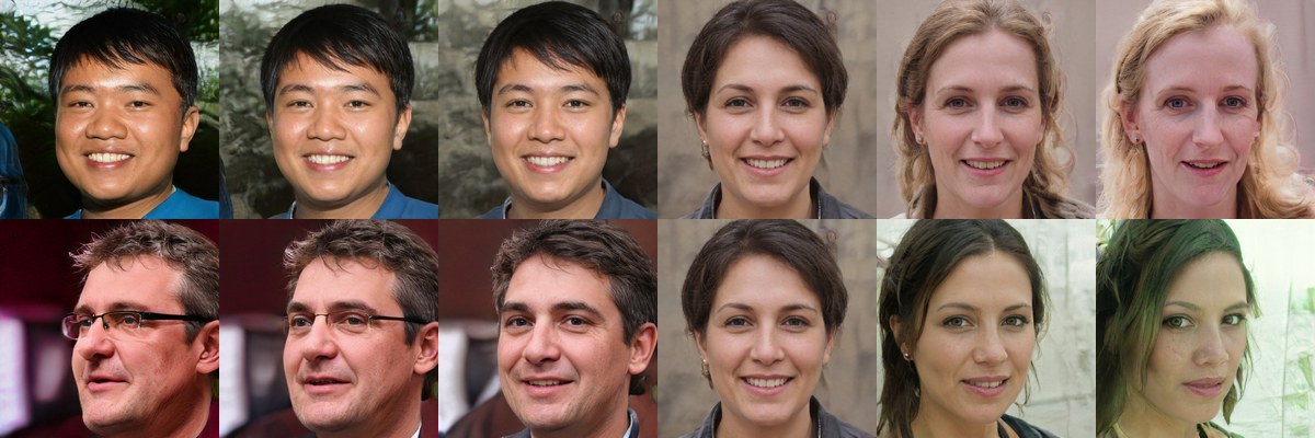
Two seeds, \(\psi\) = 1, 0.7, 0.5, 0, −0.5, −1 left to right (Karras et al. 2019, Fig. 8)
Definition (Karras et al. 2019)
- \(\bar{\mathbf{w}} = \mathbb{E}_{\mathbf{z}}[f(\mathbf{z})]\) - the center of \(\mathbf{w}\)-space, decoding to an average face (\(\psi = 0\))
- \(\mathbf{w}' = \bar{\mathbf{w}} + \psi(\mathbf{w} - \bar{\mathbf{w}})\) - every sample pulled toward the center by \(\psi < 1\)
- \(\psi < 0\): reflected through the center - every attribute flips
What it trades
- \(\psi \to 0\): samples land in the densest region - fewer artifacts, less variety, one face
- Applied at generation time - nothing about training changes
- Off the typical shell: \(\psi < 1\) moves samples toward the center of \(\mathbf{w}\)-space, where density is high and draws are rare - fidelity gained by leaving the region the prior samples
Truncated samples are atypical by construction - the trade is fidelity for the diversity the prior would have drawn.
Paired Translation Learns from Correspondence
Pix2Pix (Isola et al. 2017) - image in, image out, with aligned pairs
\[\mathcal{L} = \mathcal{L}_{\text{cGAN}}(G, D) + \lambda\, \mathbb{E}\!\left[\|y - G(\mathbf{x})\|_1\right], \qquad \lambda = 100\]
Generator: encoder-decoder with skips
- U-Net form - the segmentation architecture, generating instead of labeling
- Skips carry input detail past the bottleneck - alignment comes through the skips, not the decoder
Discriminator: PatchGAN
- Real/fake per 70 × 70 patch, averaged - texture judged locally
- 2.7M parameters against 41M for a whole-image \(D\)
The two losses split the work
- \(L_1\): gets the low frequencies right - blurry alone
- Adversarial: sharpens the texture the \(L_1\) term averages away
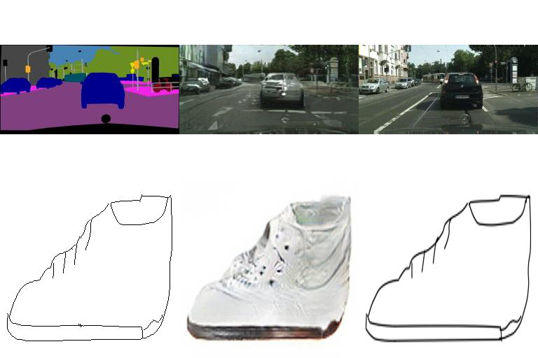
Input \(\mathbf{x}\), output \(G(\mathbf{x})\), target \(y\): Cityscapes labels to photo, edges to shoe (Isola et al. 2017, from the paper’s result sets)
Paired data is the constraint - one aligned \((\mathbf{x}, y)\) per training example.
Cycle Consistency Replaces Paired Data
CycleGAN (Zhu et al. 2017) - two domains, no pairs
- Two generators: \(G: X \to Y\), \(\;F: Y \to X\) - two discriminators \(D_X\), \(D_Y\)
\[\mathcal{L}_{\text{cyc}} = \mathbb{E}_{\mathbf{x}}\!\left[\|F(G(\mathbf{x})) - \mathbf{x}\|_1\right] + \mathbb{E}_{\mathbf{y}}\!\left[\|G(F(\mathbf{y})) - \mathbf{y}\|_1\right]\]
- Cycle consistency replaces correspondence: translate over, translate back, land at the input
Failure modes
- Semantic drift: geometry changes when only texture should
- Hidden information: \(G\) encodes the input in imperceptible high-frequency detail so that \(F\) can invert it - the cycle check passes without a semantic map (Chu et al. 2017)
- Texture bias: color moves, structure resists
Cost
- Four networks - 2× the memory of one GAN
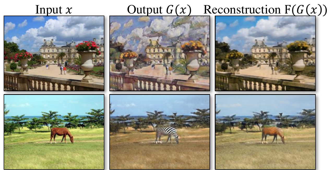
Input, \(G(\mathbf{x})\), and \(F(G(\mathbf{x}))\): Monet to photo, horse to zebra (Zhu et al. 2017, Fig. 4)
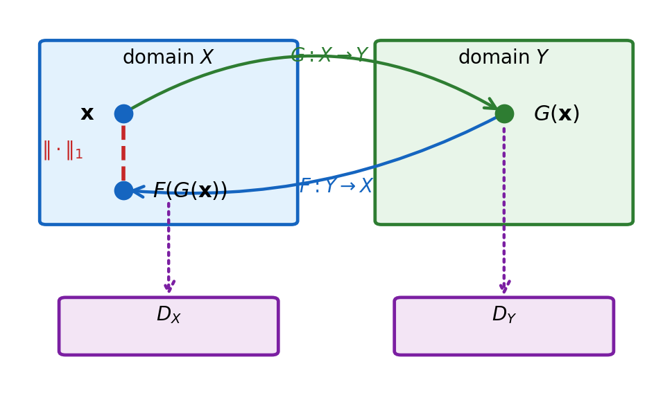
The cycle check forces \(F \circ G\) toward the identity - which invertible \(G\) satisfies it is left to the adversarial terms.
Inception Score Rewards Confident, Varied Classes
\[\text{IS} = \exp\!\left(\mathbb{E}_{\mathbf{x} \sim p_g}\!\left[\text{KL}\!\left(p(y|\mathbf{x}) \,\|\, p(y)\right)\right]\right)\]
- \(p(y|\mathbf{x})\): an ImageNet classifier’s prediction - \(p(y)\): its average over samples
- High IS: each sample confidently classified, classes varied overall
- Range: 1 to the number of classes
What it punishes
- Collapse to one class: \(p(y) \to p(y|\mathbf{x})\), KL \(\to 0\) - IS falls to its minimum
What it cannot see
- One perfect image per class, repeated: confident, varied - IS maximal, diversity gone
- Within-class variety: invisible to \(p(y|\mathbf{x})\) entirely
Scope
- Tied to the ImageNet classifier - uninformative off-domain
- Optimizing IS directly: overfits the classifier, not the data
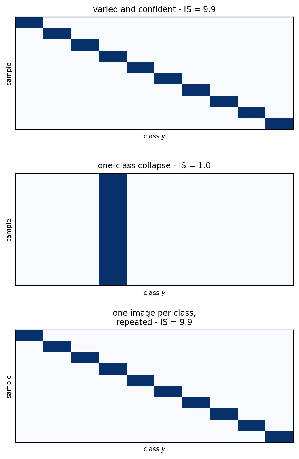
A high IS rules out class collapse and nothing else.
FID Compares Feature Distributions
\[\text{FID} = \|\boldsymbol{\mu}_r - \boldsymbol{\mu}_g\|^2 + \text{Tr}\!\left(\boldsymbol{\Sigma}_r + \boldsymbol{\Sigma}_g - 2\left(\boldsymbol{\Sigma}_r \boldsymbol{\Sigma}_g\right)^{1/2}\right)\]
Construction (Heusel et al. 2017)
- Inception features (pool3, 2048-d) of both sample sets, a Gaussian fitted to each
- FID = the Fréchet distance between the two fits - lower is better, 0 = identical fits
- Evaluation as distribution comparison - a sample set against a sample set, in kind with the objective
Against IS
- Real data enters the comparison - IS never looks at it
- A mode dropped within a class moves \(\boldsymbol{\mu}_g, \boldsymbol{\Sigma}_g\) - FID rises where IS holds still
Assumptions
- Features treated as Gaussian - two moments only
- Inherits the Inception network’s feature geometry - ImageNet-trained, ImageNet-biased
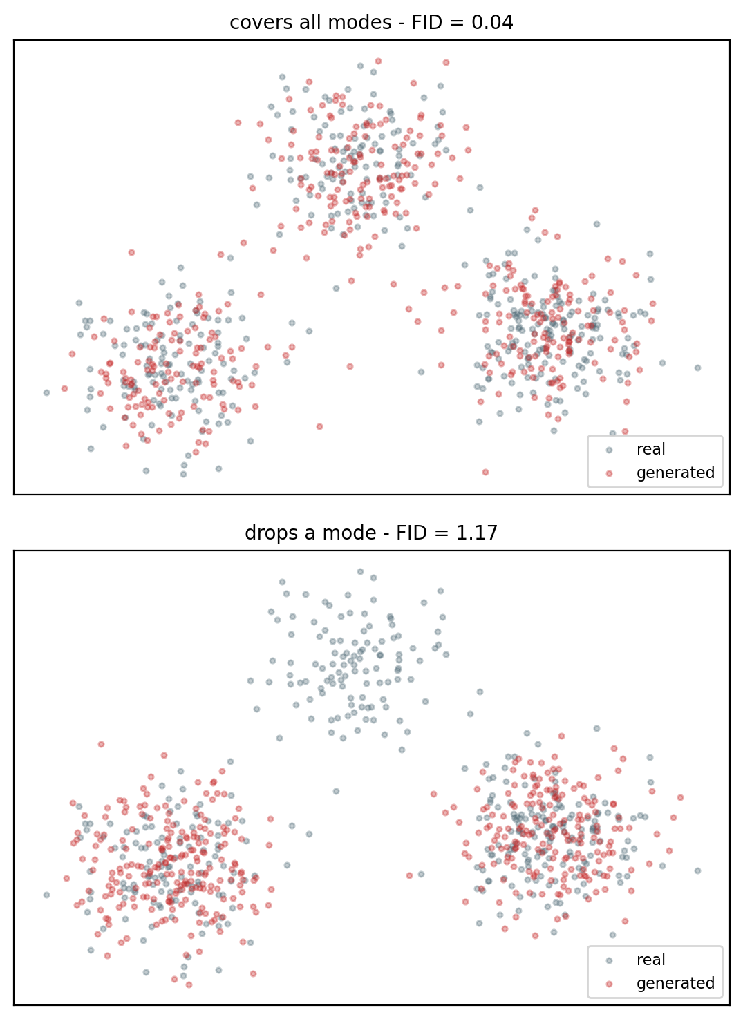
Real data enters FID and not IS - the two metrics fail on different collapses.
Precision and Recall Separate Fidelity from Diversity
Two manifolds, two fractions (Kynkäänniemi et al. 2019)
- \(\text{manifold}(S)\): the union of balls around each feature vector in \(S\), radius = distance to its \(k\)-th nearest neighbor in \(S\) (\(k = 3\))
\[\text{precision} = \frac{1}{|G|}\sum_{\mathbf{g} \in G} \mathbb{1}\!\left[\mathbf{g} \in \text{manifold}(R)\right]\]
\[\text{recall} = \frac{1}{|R|}\sum_{\mathbf{r} \in R} \mathbb{1}\!\left[\mathbf{r} \in \text{manifold}(G)\right]\]
- Precision: generated samples that land on the data - fidelity
- Recall: data that the generator covers - diversity
What FID reports as one number
- Truncation: precision up, recall down - FID moves one way and hides the trade
- Mode dropping: recall falls, precision unchanged
- Off-manifold samples: precision falls, recall unchanged
- Protocol-bound like FID: same features, same \(N\), same \(k\)
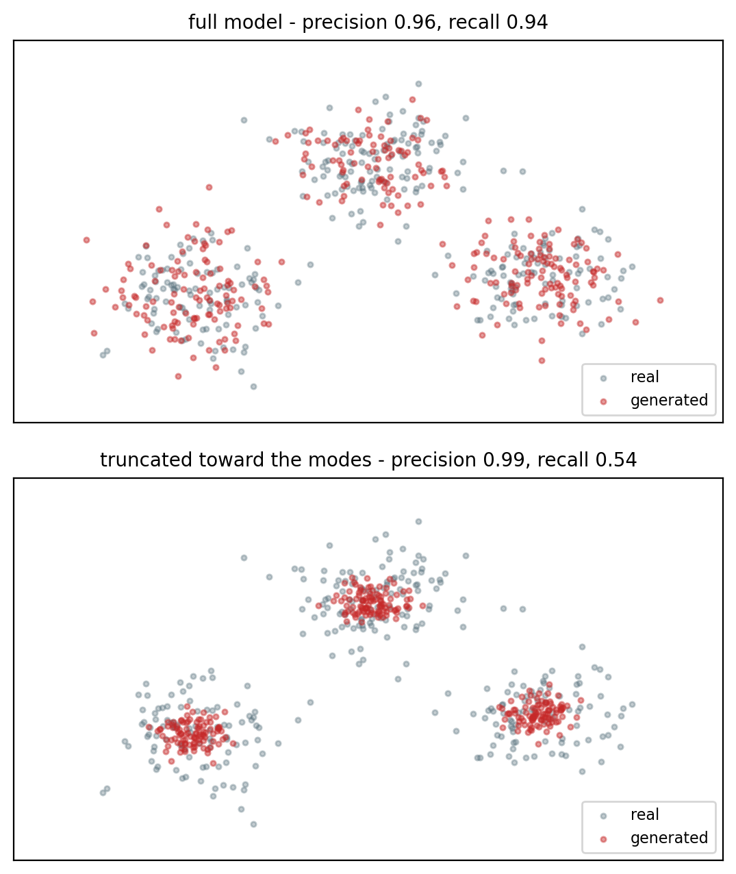
FID reports one number for a trade with two sides - truncation moves the sides in opposite directions.
An FID Is Comparable Only Under One Protocol
Sample size
- The estimate is biased upward at small \(N\) - and noisy
- Reported numbers: 50k samples standard - 10k for quick checks only
- Same \(N\) on both sides - real and generated
Everything else held fixed
- Same preprocessing and resizing path
- Same Inception weights and implementation
- Resizing and compression differences alone shift FID by more than some model differences (Parmar et al. 2022)
Reading a published FID
- Dataset, sample count, and pipeline - always stated with the number
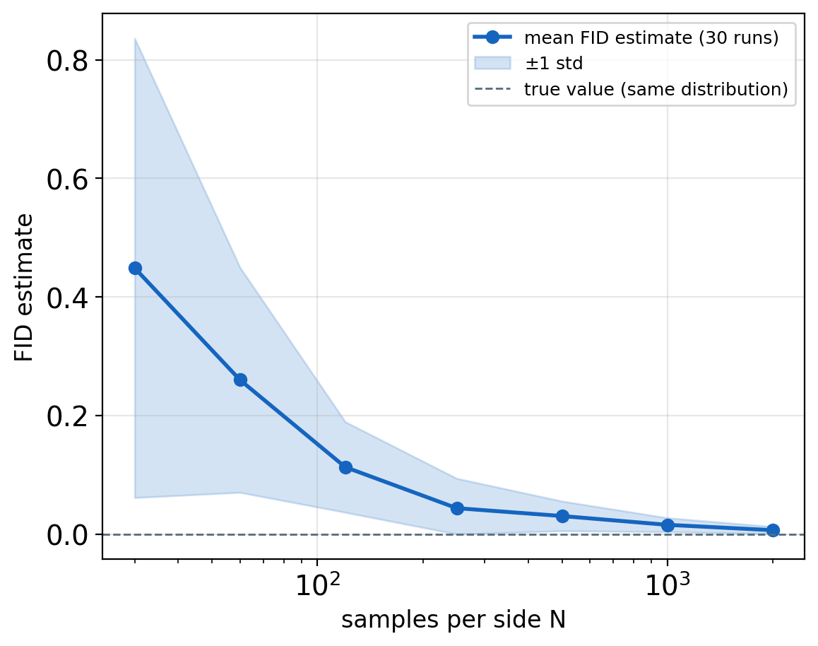
A published FID is a statement about a protocol - compare only numbers that share it.
A GAN Has No Likelihood and No Encoder
Dropping the density
- One pass per sample, sharp outputs, no partition function, no chain - and no \(\log p_g(\mathbf{x})\)
- Every score above is a proxy computed from samples - IS, FID, precision and recall
Three things a sampler cannot do
- Score held-out data: no likelihood, so no model comparison from the model itself
- Encode: given \(\mathbf{x}\), no \(\mathbf{z}\) - inversion needs optimization or a second network
- Report progress: the game’s losses oscillate - stopping falls back on the proxies
Third option
- Keep the latent and the sampler - add an encoder and a lower bound on \(\log p(\mathbf{x})\), paying with a bound in place of the likelihood
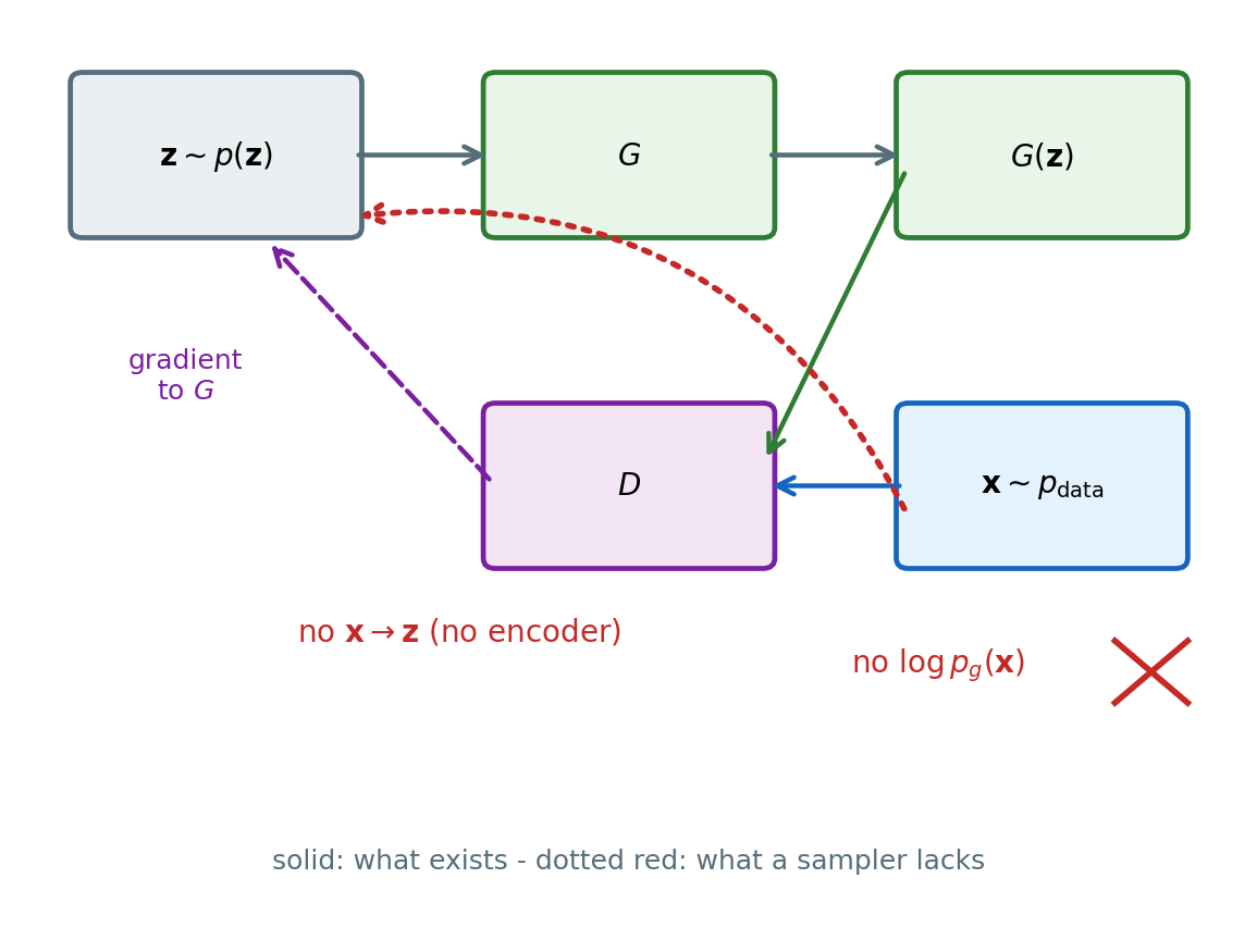
A sampler without a density can be judged only by its samples - the encoder and the likelihood bound are what the next family adds.
A Latent Variable Model Has a Density and No \(Z\)
Two families so far
- Energy: \(p(\mathbf{x}) = e^{-E(\mathbf{x})}/Z\) - a density, normalized over all of \(\mathbf{x}\)-space, and \(Z\) cannot be computed
- Sampler only: \(\mathbf{x} = G(\mathbf{z})\) - no density, so no \(Z\) and nothing to score but samples
Latent variable model
- \(p(\mathbf{x}) = \int p(\mathbf{x}|\mathbf{z})\, p(\mathbf{z})\, d\mathbf{z}\) - every factor normalized, no \(Z\), and the integral over \(\mathbf{z}\) remains
- A simple prior and a simple conditional give a complex marginal - the shape comes from the decoder’s nonlinearity
- A density for training and scoring, a posterior for inference
Cost
- The integral has no closed form - training uses a bound on \(\log p(\mathbf{x})\), not \(\log p(\mathbf{x})\) itself
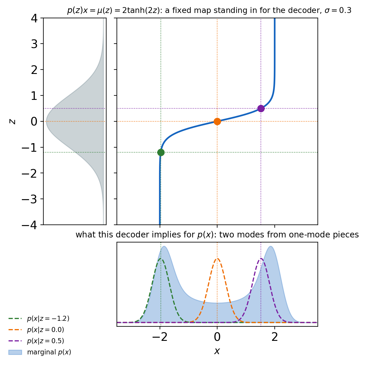
All learned structure is in the decoder - the integral over \(\mathbf{z}\) is what remains intractable.
Training Needs the Marginal, Inference Needs the Posterior
The marginal \(p_{\boldsymbol{\theta}}(\mathbf{x})\)
\[p_{\boldsymbol{\theta}}(\mathbf{x}) = \int p_{\boldsymbol{\theta}}(\mathbf{x}|\mathbf{z})\, p(\mathbf{z})\, d\mathbf{z}\]
- Maximum likelihood trains on \(\log p_{\boldsymbol{\theta}}(\mathbf{x})\) - the forward-KL objective, data in the first argument
- Held-out \(\log p_{\boldsymbol{\theta}}(\mathbf{x})\): the score a GAN cannot produce
The posterior \(p_{\boldsymbol{\theta}}(\mathbf{z}|\mathbf{x})\)
\[p_{\boldsymbol{\theta}}(\mathbf{z}|\mathbf{x}) = \frac{p_{\boldsymbol{\theta}}(\mathbf{x}|\mathbf{z})\, p(\mathbf{z})}{p_{\boldsymbol{\theta}}(\mathbf{x})}\]
- The latent for a given \(\mathbf{x}\) - the encoding direction a GAN does not have
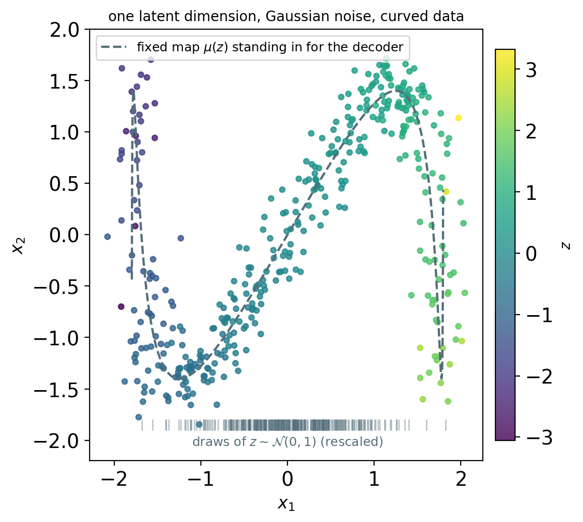
- Its shape is set by the decoder - non-Gaussian and correlated whenever \(\boldsymbol{\mu}_{\boldsymbol{\theta}}\) is nonlinear
Shared denominator
- The marginal is the posterior’s normalizer - both require the same integral
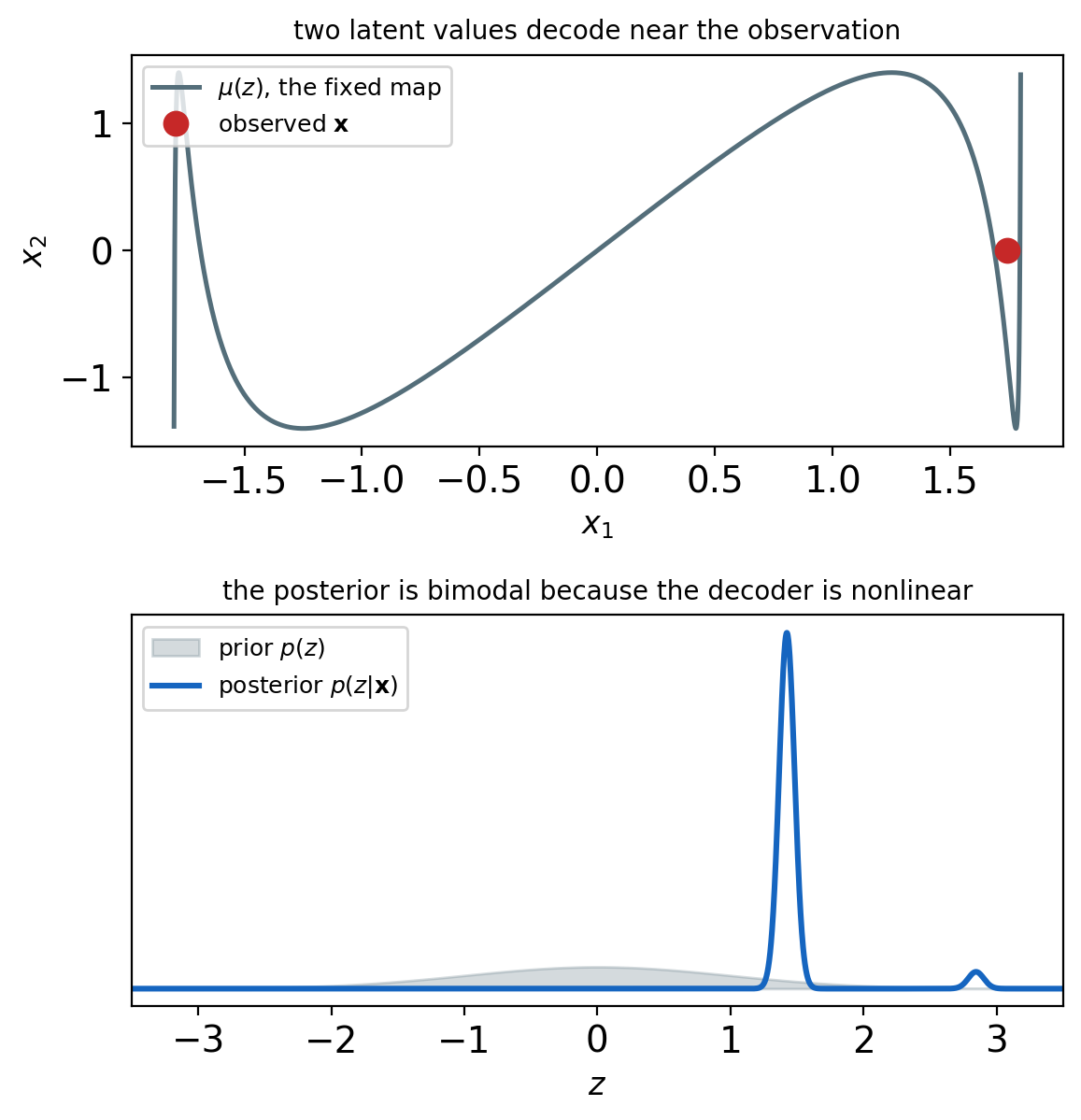
The likelihood and the posterior require the same integral over \(\mathbf{z}\).
The Integral over \(\mathbf{z}\) Is Intractable for a Network Decoder
No closed form
- \(\int \mathcal{N}(\mathbf{x}; \boldsymbol{\mu}_{\boldsymbol{\theta}}(\mathbf{z}), \sigma^2 \mathbf{I})\, \mathcal{N}(\mathbf{z}; \mathbf{0}, \mathbf{I})\, d\mathbf{z}\) - no analytic integral for a nonlinear \(\boldsymbol{\mu}_{\boldsymbol{\theta}}\)
- Quadrature over \(\mathbf{z}\): exponential in \(k\)
Monte Carlo from the prior fails
- \(p_{\boldsymbol{\theta}}(\mathbf{x}) \approx \frac{1}{N}\sum_i p_{\boldsymbol{\theta}}(\mathbf{x}|\mathbf{z}_i)\), \(\;\mathbf{z}_i \sim p(\mathbf{z})\) - unbiased, with variance too large to use
- Almost every prior draw decodes far from \(\mathbf{x}\) - \(p_{\boldsymbol{\theta}}(\mathbf{x}|\mathbf{z}_i) \approx 0\) for all but a vanishing fraction
- Effective sample size falls exponentially in \(k\) - the same failure as rejection sampling
Requirement
- Draws from where \(p_{\boldsymbol{\theta}}(\mathbf{x}|\mathbf{z})\) is large - draws from the posterior
- The posterior requires the marginal - the same integral
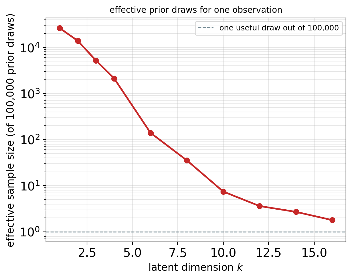
Training requires the posterior and cannot compute it - variational inference replaces it with an approximation.
A Tractable Family Stands In for the Posterior
Substitution
- \(q_{\boldsymbol{\phi}}(\mathbf{z}|\mathbf{x})\) from a fixed family replaces \(p_{\boldsymbol{\theta}}(\mathbf{z}|\mathbf{x})\) - the standard family is a diagonal Gaussian, \(\mathcal{N}(\boldsymbol{\mu}_{\boldsymbol{\phi}}(\mathbf{x}), \text{diag}\, \boldsymbol{\sigma}^2_{\boldsymbol{\phi}}(\mathbf{x}))\)
- \(\boldsymbol{\phi}\) chosen to make \(q\) close to the posterior - the objective must not require \(p_{\boldsymbol{\theta}}(\mathbf{x})\)
Only reverse KL is computable
- \(\text{KL}(q \,\|\, p(\mathbf{z}|\mathbf{x}))\): an expectation under \(q\) - samples available
- \(\text{KL}(p(\mathbf{z}|\mathbf{x}) \,\|\, q)\): an expectation under the posterior - no samples, so no estimate
- Reverse KL, model in the first argument - the direction that concentrates on one mode
What the family cannot represent
- The true posterior is non-Gaussian and correlated whenever the decoder is nonlinear
- A diagonal Gaussian under reverse KL: one mode, and variances from the posterior’s precision diagonal - narrower than the posterior’s own marginals
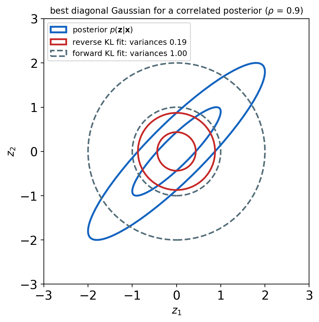
The computable direction is reverse KL, and reverse KL fits one mode too narrowly - the approximation error has a known sign.
The ELBO Is \(\log p(\mathbf{x})\) Minus the Posterior Gap
One identity, for any \(q\)
\[\log p_{\boldsymbol{\theta}}(\mathbf{x}) = \underbrace{\mathbb{E}_{q_{\boldsymbol{\phi}}(\mathbf{z}|\mathbf{x})}\!\left[\log \frac{p_{\boldsymbol{\theta}}(\mathbf{x}, \mathbf{z})}{q_{\boldsymbol{\phi}}(\mathbf{z}|\mathbf{x})}\right]}_{\mathcal{L}(\boldsymbol{\theta}, \boldsymbol{\phi}; \mathbf{x})} + \underbrace{\text{KL}\!\left(q_{\boldsymbol{\phi}}(\mathbf{z}|\mathbf{x}) \,\|\, p_{\boldsymbol{\theta}}(\mathbf{z}|\mathbf{x})\right)}_{\geq 0}\]
- Proof: write \(p(\mathbf{x}, \mathbf{z}) = p(\mathbf{x})\, p(\mathbf{z}|\mathbf{x})\) inside the expectation - \(\log p(\mathbf{x})\) factors out, the remainder is the KL
- \(\mathcal{L} \leq \log p_{\boldsymbol{\theta}}(\mathbf{x})\), equality iff \(q\) equals the posterior - the evidence lower bound, ELBO, evidence being the name for \(p_{\boldsymbol{\theta}}(\mathbf{x})\)
Same bound by Jensen
- \(\log \mathbb{E}_q[p(\mathbf{x}, \mathbf{z}) / q] \geq \mathbb{E}_q[\log(p(\mathbf{x}, \mathbf{z}) / q)]\) - concavity of \(\log\); the gap is the KL above
Training form
\[\mathcal{L} = \mathbb{E}_{q_{\boldsymbol{\phi}}(\mathbf{z}|\mathbf{x})}\!\left[\log p_{\boldsymbol{\theta}}(\mathbf{x}|\mathbf{z})\right] - \text{KL}\!\left(q_{\boldsymbol{\phi}}(\mathbf{z}|\mathbf{x}) \,\|\, p(\mathbf{z})\right)\]
- Every term computable: \(q\) samples, the decoder likelihood, the prior - no \(p_{\boldsymbol{\theta}}(\mathbf{x})\) anywhere
- Maximized over \(\boldsymbol{\phi}\): \(q\) approaches the posterior. Over \(\boldsymbol{\theta}\): the decoder changes the posterior too, so the gap can grow while the bound rises
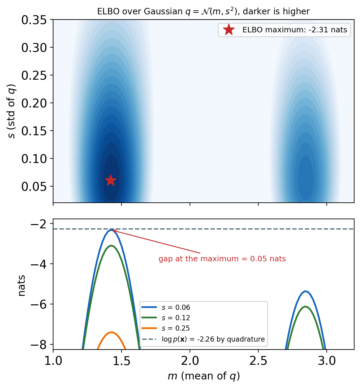
The bound is exact minus a KL that is never negative - maximizing it over \(q\) is the same problem as fitting the posterior.
Both the Bound and \(\log p_{\boldsymbol{\theta}}(\mathbf{x})\) Move During Training
Two parameter sets, two effects
- \(\boldsymbol{\phi}\)-steps: \(q\) moves toward the posterior - the gap \(\text{KL}(q \,\|\, p_{\boldsymbol{\theta}}(\mathbf{z}|\mathbf{x}))\) shrinks, the bound rises toward a fixed \(\log p_{\boldsymbol{\theta}}(\mathbf{x})\)
- \(\boldsymbol{\theta}\)-steps: the decoder changes - \(\log p_{\boldsymbol{\theta}}(\mathbf{x})\) itself rises, and the posterior it defines moves, so the gap can widen at the same time
What the training loop sees
- Only the bound - \(\log p_{\boldsymbol{\theta}}(\mathbf{x})\) is never computed, so the gap is never observed directly
- A rising bound is consistent with a rising likelihood and with a closing gap - the curve alone does not say which
What the number at the end means
- The final \(\mathcal{L}\) on held-out data is a lower bound on held-out \(\log p_{\boldsymbol{\theta}}(\mathbf{x})\) - the model’s likelihood is at least this, and the shortfall is the posterior gap
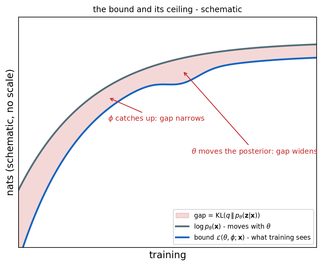
Training reports the bound and never the gap - the bound’s rise is the sum of two movements it cannot tell apart.
One Encoder Serves Every Data Point
Per-datapoint inference
- Classical variational inference: one optimization of \((\mathbf{m}_i, \mathbf{s}_i)\) per \(\mathbf{x}_i\) - \(2k\) free parameters per point, restarted for every new \(\mathbf{x}\)
Amortized inference
- One network: \(\mathbf{x} \mapsto (\boldsymbol{\mu}_{\boldsymbol{\phi}}(\mathbf{x}), \boldsymbol{\sigma}_{\boldsymbol{\phi}}(\mathbf{x}))\) - the encoder
- Shared \(\boldsymbol{\phi}\) across the dataset - inference for a new \(\mathbf{x}\) is one forward pass
- The variational autoencoder is this pair: encoder \(q_{\boldsymbol{\phi}}\), decoder \(p_{\boldsymbol{\theta}}\), trained together on \(\mathcal{L}\)
Amortization gap
- The encoder’s \(q\) for a given \(\mathbf{x}\) is worse than the best \(q\) in the family for that \(\mathbf{x}\) - a second gap under the bound (Cremer et al. 2018)
- Total slack: \(\log p(\mathbf{x}) - \mathcal{L} = \text{family gap} + \text{amortization gap}\)
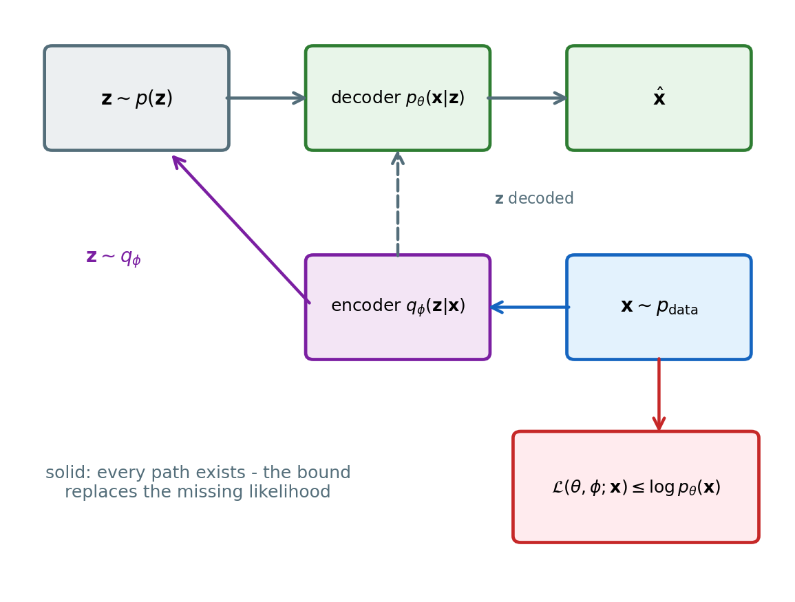
The encoder is the inverse path a sampler lacked and the bound is the number a sampler could not report - both approximate, by the two gaps.
The KL Term Is Information Plus Prior Mismatch
Aggregate posterior
- \(q_{\boldsymbol{\phi}}(\mathbf{z}) = \frac{1}{N}\sum_i q_{\boldsymbol{\phi}}(\mathbf{z}|\mathbf{x}_i)\) - the code distribution over the whole dataset
The regularizer, averaged (Hoffman and Johnson 2016)
\[\frac{1}{N}\sum_i \text{KL}\!\left(q(\mathbf{z}|\mathbf{x}_i) \,\|\, p(\mathbf{z})\right) = \underbrace{I_q(\mathbf{x}; \mathbf{z})}_{\text{code carries information}} + \underbrace{\text{KL}\!\left(q(\mathbf{z}) \,\|\, p(\mathbf{z})\right)}_{\text{aggregate differs from the prior}}\]
- Proof: add and subtract \(\log q(\mathbf{z})\) inside the KL - the mutual information is the average KL of each \(q(\mathbf{z}|\mathbf{x}_i)\) to the aggregate
What the objective penalizes
- Information in the code, \(I_q(\mathbf{x};\mathbf{z})\): bounded by \(\log N\), each nat charged at full weight
- Mismatch between the aggregate and the prior: regions of \(\mathbf{z}\) the prior samples that no data point encodes to
What follows
- A code that carries nothing costs nothing - \(I_q \to 0\) is a valid optimum of the regularizer alone
- Reweighting the KL term reweights both, not one - posterior collapse and the β-VAE trade both come from this split
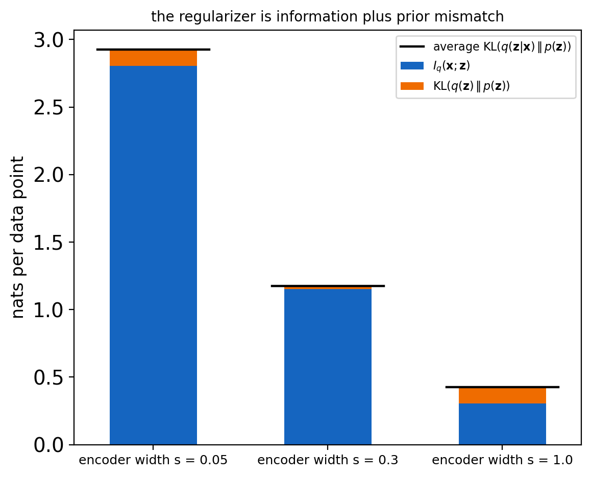
The KL term is two costs, information in the code and mismatch with the prior, with one weight in front of both.
The Gaussian KL Has a Closed Form
Encoder output against the prior
- \(q_{\boldsymbol{\phi}}(\mathbf{z}|\mathbf{x}) = \mathcal{N}(\boldsymbol{\mu}, \text{diag}\, \boldsymbol{\sigma}^2)\), \(\;p(\mathbf{z}) = \mathcal{N}(\mathbf{0}, \mathbf{I})\)
\[\text{KL}\!\left(q \,\|\, p\right) = \frac{1}{2}\sum_{j=1}^{k}\left(\mu_j^2 + \sigma_j^2 - \log \sigma_j^2 - 1\right)\]
From the general Gaussian formula
\[\text{KL}\!\left(\mathcal{N}_1 \,\|\, \mathcal{N}_2\right) = \frac{1}{2}\left[\text{tr}\!\left(\boldsymbol{\Sigma}_2^{-1}\boldsymbol{\Sigma}_1\right) + (\boldsymbol{\mu}_2 - \boldsymbol{\mu}_1)^\top \boldsymbol{\Sigma}_2^{-1} (\boldsymbol{\mu}_2 - \boldsymbol{\mu}_1) - k + \log \frac{|\boldsymbol{\Sigma}_2|}{|\boldsymbol{\Sigma}_1|}\right]\]
- With \(\boldsymbol{\mu}_2 = \mathbf{0}\), \(\boldsymbol{\Sigma}_2 = \mathbf{I}\), \(\boldsymbol{\Sigma}_1\) diagonal: the trace is \(\sum \sigma_j^2\), the quadratic is \(\sum \mu_j^2\), the log-determinant is \(-\sum \log \sigma_j^2\)
Per dimension
- \(\mu_j^2\): distance of the code’s mean from the prior’s
- \(\sigma_j^2 - \log \sigma_j^2 - 1\): zero at \(\sigma_j = 1\), positive on either side - a variance both larger and smaller than the prior’s costs
- Minimum zero at \(\mu_j = 0\), \(\sigma_j = 1\) - a dimension that matches the prior is free
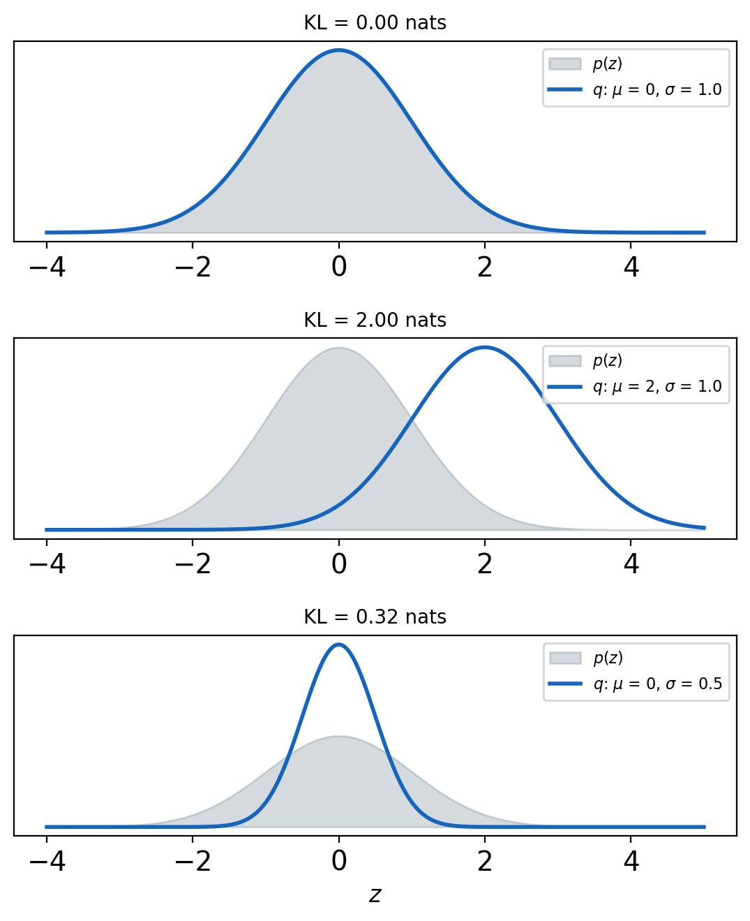
The regularizer is a sum of per-dimension costs, each zero exactly when that dimension matches the prior.
Two Estimators for the Gradient of an Expectation
Gradient of an expectation
- \(\nabla_{\boldsymbol{\phi}}\, \mathbb{E}_{q_{\boldsymbol{\phi}}(\mathbf{z})}[f(\mathbf{z})]\) with \(\boldsymbol{\phi}\) in the distribution, not in \(f\) - the derivative cannot pass inside the expectation as written
Score-function estimator
\[\nabla_{\boldsymbol{\phi}} \int q_{\boldsymbol{\phi}} f = \int f\, \nabla_{\boldsymbol{\phi}} q_{\boldsymbol{\phi}} = \int q_{\boldsymbol{\phi}}\, f\, \nabla_{\boldsymbol{\phi}} \log q_{\boldsymbol{\phi}} = \mathbb{E}_{q_{\boldsymbol{\phi}}}\!\left[f(\mathbf{z})\, \nabla_{\boldsymbol{\phi}} \log q_{\boldsymbol{\phi}}(\mathbf{z})\right]\]
- Uses only values of \(f\) - works for any \(q\), discrete included
- Variance scales with the magnitude of \(f\), not with its slope
Pathwise estimator - reparameterization
\[\mathbf{z} = g(\boldsymbol{\epsilon}, \boldsymbol{\phi}) = \boldsymbol{\mu}_{\boldsymbol{\phi}} + \boldsymbol{\sigma}_{\boldsymbol{\phi}} \odot \boldsymbol{\epsilon}, \quad \boldsymbol{\epsilon} \sim \mathcal{N}(\mathbf{0}, \mathbf{I}) \qquad \nabla_{\boldsymbol{\phi}}\, \mathbb{E}_{\boldsymbol{\epsilon}}[f(g(\boldsymbol{\epsilon}, \boldsymbol{\phi}))] = \mathbb{E}_{\boldsymbol{\epsilon}}\!\left[\nabla_{\mathbf{z}} f \cdot \frac{\partial g}{\partial \boldsymbol{\phi}}\right]\]
- The randomness moves to \(\boldsymbol{\epsilon}\), which has no parameters - the derivative passes inside
- Uses \(\nabla_{\mathbf{z}} f\) - variance scales with the slope of \(f\), not its magnitude
Which families reparameterize
- Location-scale (Gaussian, Laplace, logistic) and any inverse-CDF sampler
- Not categorical, not discrete - the cases Gumbel-softmax and the straight-through estimator handle
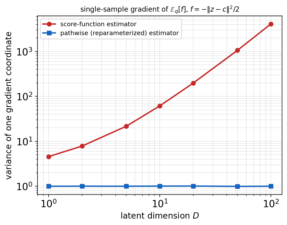
Both estimators are unbiased - the pathwise one uses the slope of \(f\) and its variance does not grow with the latent dimension.
Reparameterization Makes the ELBO a Standard Backpropagation Problem
One forward pass per data point
- One sample of \(\boldsymbol{\epsilon}\) per data point - the pathwise variance is low enough
- KL in closed form, reconstruction by Monte Carlo with one draw
The log-variance head
- A linear head can produce any real number - \(\sigma^2 = e^{\text{head}}\) is positive without a constraint
- Clamped to \([-10, 10]\) in practice - \(\sigma^2\) from \(4.5 \times 10^{-5}\) to \(2.2 \times 10^{4}\), wide enough for any encoder and a guard on the \(e^{\log\sigma^2}\) term of the KL
Cost
- Encoder pass, decoder pass, and their backward passes - four network evaluations per update, against six for a GAN and about 120 for a truncated EBM
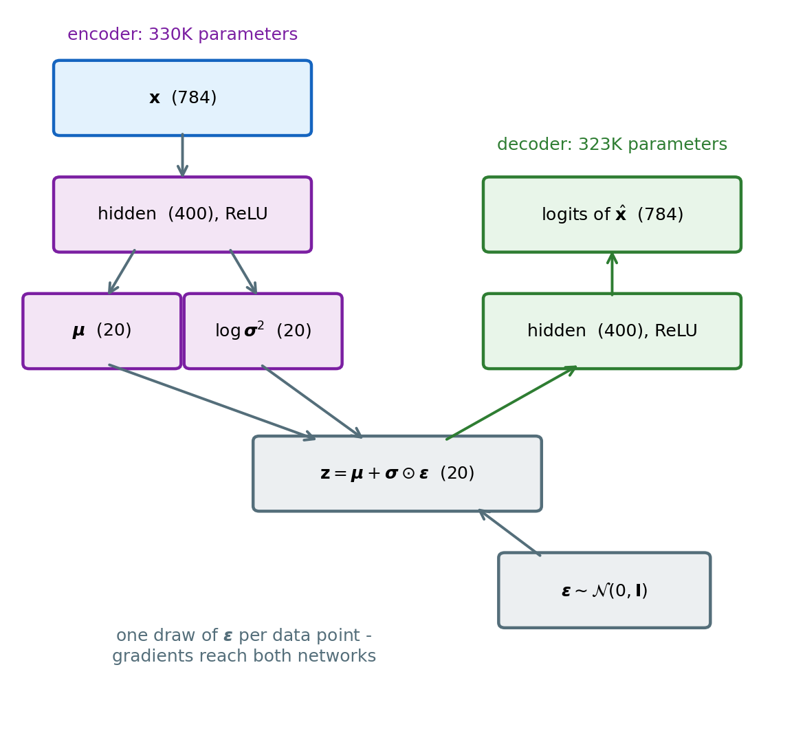
The sampling step sits between two ordinary networks - with the noise drawn outside, the whole graph is differentiable end to end.
The Output Distribution Sets the Reconstruction Loss
Bernoulli - binary data
- \(p(\mathbf{x}|\mathbf{z}) = \prod_i \text{Bernoulli}(x_i \,|\, \pi_i(\mathbf{z}))\), decoder outputs logits - the loss is binary cross-entropy with logits
Gaussian with fixed \(\sigma^2\) - continuous data
\[-\log p(\mathbf{x}|\mathbf{z}) = \frac{1}{2\sigma^2}\|\mathbf{x} - \boldsymbol{\mu}_{\boldsymbol{\theta}}(\mathbf{z})\|^2 + \text{const}\]
- \(\sigma^2\) is the weight of reconstruction against the KL term - plain
mse_losswithreduction='sum'is this loss at \(\sigma^2 = \tfrac{1}{2}\), not at unit variance - Squared error and a single mean: where the conditional has several modes, the optimal \(\boldsymbol{\mu}\) is their average - the blur of Gaussian decoders is this average, not a defect of the network
Gaussian with learned \(\sigma^2\)
- Per-pixel \(\sigma_i^2 \to 0\) on any pixel the mean fits exactly: \(-\log p \to -\infty\) - the likelihood is unbounded, and gradient descent moves toward it
- Used with a floor on \(\sigma^2\) or one shared \(\sigma^2\) per image (Rybkin et al. 2021)
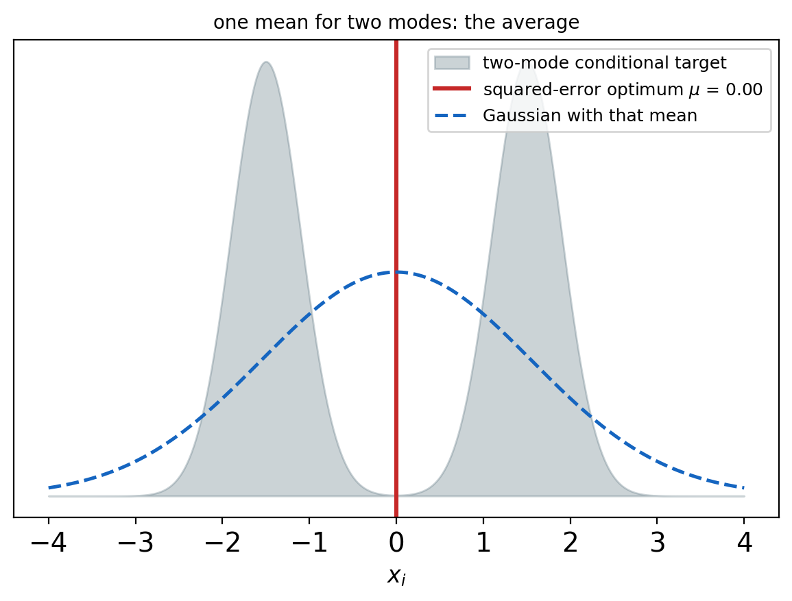
The likelihood chosen for \(p(\mathbf{x}|\mathbf{z})\) is the reconstruction loss and its scale is the KL weight - two decisions made by one line.
Reconstruction Falls First, Then the KL Term Rises
Setup
- 600 points on a curve in the plane, Gaussian noise \(\sigma = 0.18\) (left panel)
- Encoder and decoder of two hidden layers, latent \(k = 2\) - Gaussian decoder, \(\sigma\) fixed
- Four runs differing only in the KL weight \(\beta\) - \(\beta = 1\) is the ELBO
At \(\beta = 1\)
- Reconstruction falls first - the KL rises as the code starts to carry information
- \(-\mathcal{L}\) decreases throughout - a loss that tracks the objective
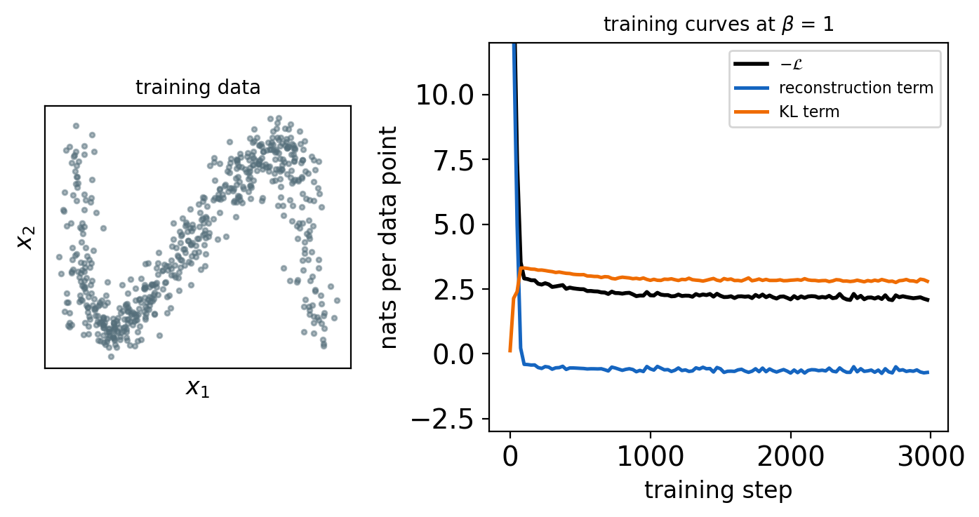
A loss that decreases is what the bound provides - the adversarial game had no such curve.
Every Nat in the Code Appears in the KL Term
KL per dimension, four runs
- Both dimensions carry information at low \(\beta\) - a curve embedded in the plane uses two coordinates cheaply
- Higher \(\beta\) lowers every dimension’s share
- At \(\beta = 30\) the first dimension sits at zero - collapsed to the prior, ignored by the decoder
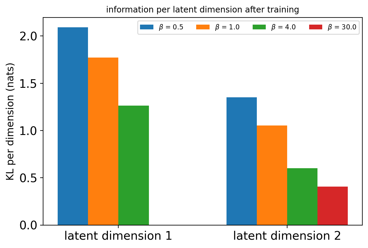
The objective prices information, not dimensions - a dimension the decoder ignores costs nothing.
Samples Are Good Only Where Encoded Data Is Nearby
Two views of one latent space
- Encoded training data: \(\boldsymbol{\mu}_{\boldsymbol{\phi}}(\mathbf{x}_i)\) for every point - where the data lands in \(\mathbf{z}\)
- Decoded prior draws: \(\boldsymbol{\mu}_{\boldsymbol{\theta}}(\mathbf{z})\) for \(\mathbf{z} \sim \mathcal{N}(\mathbf{0}, \mathbf{I})\) - what the model generates
A working model
- The encoded data fills the prior - no empty region under the bell
- Prior draws land on the data - the decoder is trained wherever the prior has mass
Holes
- A region of the prior with no encoded data - the decoder was never trained there, and the prior draws from it anyway
- The KL term is the only part of the objective that penalizes holes
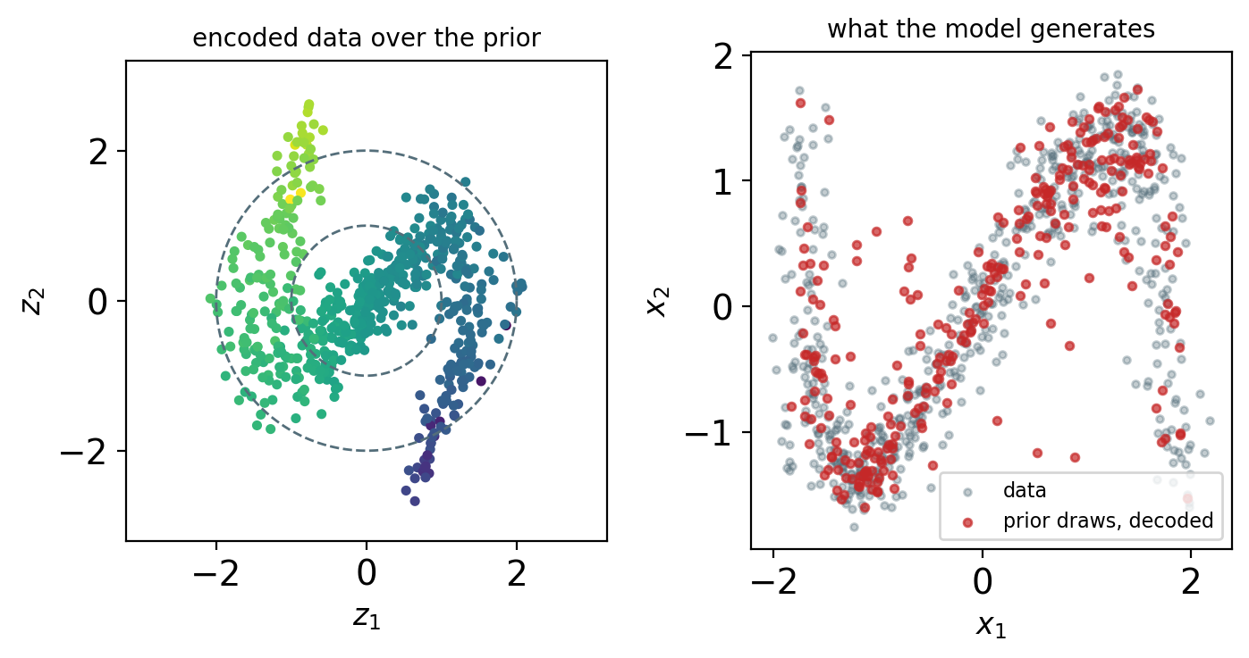
Sample quality depends on the encoded data filling the prior - nothing but the KL term asks for that.
Posterior Collapse: The Code Carries Nothing
Collapse
- \(q_{\boldsymbol{\phi}}(\mathbf{z}|\mathbf{x}) = p(\mathbf{z})\) for every \(\mathbf{x}\) - KL term zero, no information in the code
- The decoder ignores \(\mathbf{z}\) and models \(p(\mathbf{x})\) on its own - every input reconstructs to the same output
Why the objective permits it
- The KL term alone is minimized by a code that carries nothing
- Only reconstruction pays for information - if the decoder fits the data without \(\mathbf{z}\), no information is worth its cost
- When: a decoder strong enough on its own (autoregressive decoders), or early training, when the KL gradient outweighs a poor decoder (Bowman et al. 2016)
Treatments
- Warm-up: the KL weight raised from 0 to 1 over the first epochs (Bowman et al. 2016)
- Free bits: no penalty below a KL floor per dimension (Kingma et al. 2016)
- A weaker decoder, or one that cannot reach \(p(\mathbf{x})\) without \(\mathbf{z}\) (Chen et al. 2017)
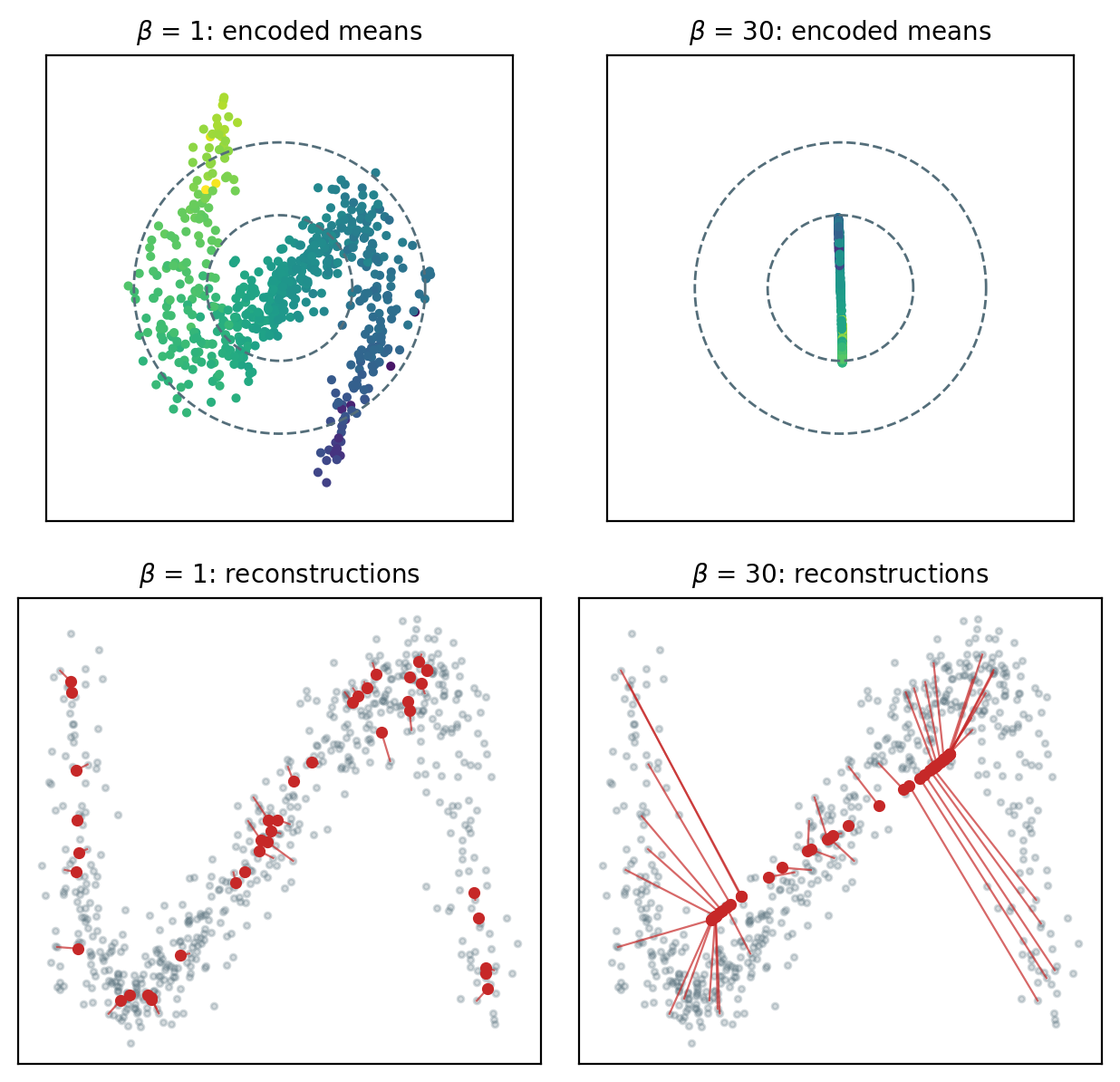
Watch the KL per dimension - a dimension at zero carries nothing, and collapse is a valid optimum of the KL term alone.
\(\beta\) Reweights Information Against Reconstruction
The objective (Higgins et al. 2017)
\[\mathcal{L}_\beta = \mathbb{E}_{q}\!\left[\log p_{\boldsymbol{\theta}}(\mathbf{x}|\mathbf{z})\right] - \beta\, \text{KL}\!\left(q_{\boldsymbol{\phi}}(\mathbf{z}|\mathbf{x}) \,\|\, p(\mathbf{z})\right)\]
- \(\beta = 1\): the bound - \(\beta > 1\): less information in the code, coarser reconstructions - \(\beta < 1\): more information, closer to a plain autoencoder
- \(\beta\) multiplies both parts of the KL term: the information in the code and the mismatch with the prior
- With a Gaussian decoder, \(\beta\) and \(\sigma^2\) are one parameter: \(\mathcal{L}_\beta / \beta\) is the bound at noise variance \(\beta \sigma^2\)
The disentanglement claim
- Higher \(\beta\) pushes the latent dimensions toward independence - reported as one factor per dimension on synthetic data with known factors
- Not guaranteed: without extra assumptions no unsupervised method identifies the factors, and the scores vary more across random seeds than across \(\beta\) (Locatello et al. 2019)
What is guaranteed
- A rate-distortion trade: each \(\beta\) picks one point on the curve of reconstruction error against information in the code
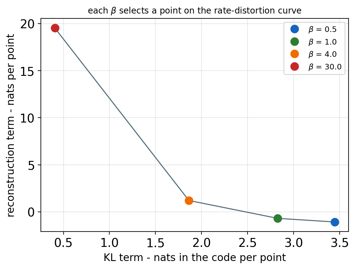
\(\beta\) sets a point on the rate-distortion curve - disentanglement is something some data show at some \(\beta\), not a consequence of the objective.
A Hierarchy of Latents Splits the Code by Scale
Model
\[p(\mathbf{x}, \mathbf{z}_1, \dots, \mathbf{z}_L) = p(\mathbf{x}|\mathbf{z}_1)\, p(\mathbf{z}_1|\mathbf{z}_2) \cdots p(\mathbf{z}_{L-1}|\mathbf{z}_L)\, p(\mathbf{z}_L)\]
- Top layer: coarse structure - lower layers: detail, conditioned on the layer above
- One KL term per layer, each against the layer above - only the top layer keeps a fixed prior
Inference top-down (Sønderby et al. 2016)
- A bottom-up pass computes features of \(\mathbf{x}\) at every level - a top-down pass forms \(q(\mathbf{z}_l | \mathbf{z}_{l+1}, \mathbf{x})\) from those features and the generative path
- \(q\) and \(p\) share the top-down network - each layer’s posterior is a correction to its prior
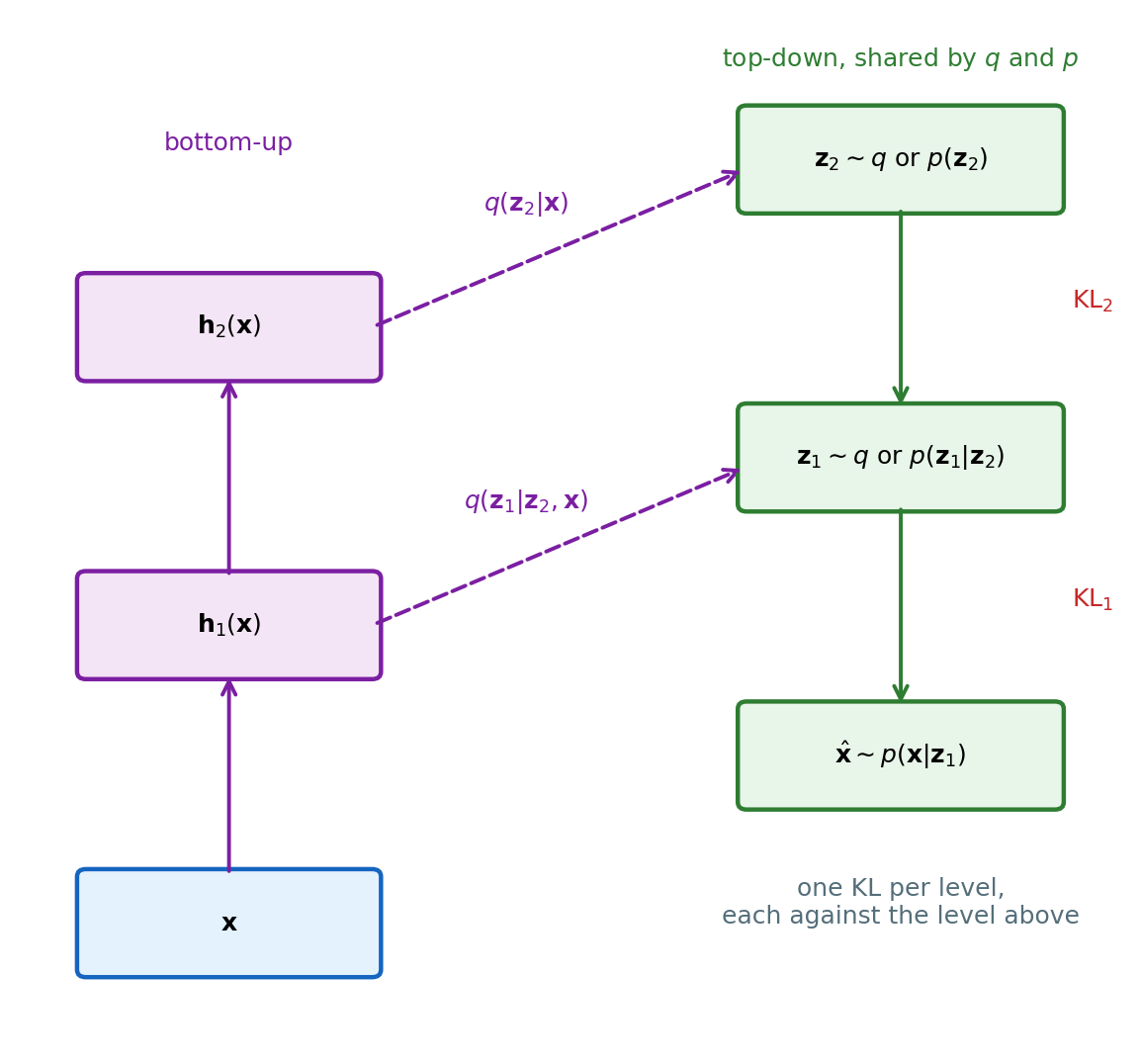
Every prior but the top one is learned - each layer is generated from the layer above it.
VQ-VAE Replaces the Gaussian Code with a Code-Book Index
Quantization in the middle (van den Oord et al. 2017)
- Encoder output \(\mathbf{z}_e = f_{\boldsymbol{\phi}}(\mathbf{x})\), continuous - snapped to the nearest of \(K\) code-book vectors: \(\mathbf{z}_q = \mathbf{e}_k\), \(k = \arg\min_j \|\mathbf{z}_e - \mathbf{e}_j\|\)
- Decoder reads \(\mathbf{z}_q\) - the code for \(\mathbf{x}\) is the index \(k\), \(\log_2 K\) bits per position
Loss, three terms
\[\mathcal{L}_{\text{VQ}} = -\log p_{\boldsymbol{\theta}}(\mathbf{x}|\mathbf{z}_q) + \|\text{sg}[\mathbf{z}_e] - \mathbf{e}_k\|^2 + \beta\, \|\mathbf{z}_e - \text{sg}[\mathbf{e}_k]\|^2\]
- Reconstruction; the code-book vector moved toward the encoder output; the encoder output moved toward its code-book vector - \(\text{sg}\) stops the gradient
- The argmin has no gradient: the decoder’s gradient at \(\mathbf{z}_q\) is copied to \(\mathbf{z}_e\) unchanged - the straight-through estimator, the discrete counterpart of reparameterization
What the KL term becomes
- Uniform prior over \(K\) indices and a deterministic posterior: \(\text{KL} = \log K\), a constant - nothing in the objective moves the code toward the prior
- No posterior collapse, but a failure of its own: a few indices used, the rest never assigned and so never updated
Generation needs a second model
- Prior draws are uniform indices - samples need a learned \(p(k_1, \dots, k_M)\) over the index grid, trained afterward (an autoregressive model in the paper)
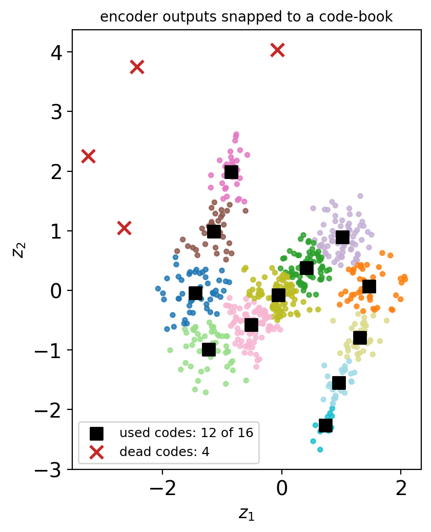
A discrete code replaces the Gaussian KL with a constant and reparameterization with a copied gradient - and fails by leaving codes unused.
Sampling a Token Breaks the Gradient Path
Where the graph breaks
- \(G\) emits logits \(\boldsymbol{\ell}\) over a vocabulary - a token is sampled, \(D\) reads tokens (with images, \(D\) read \(G\)’s output directly)
- \(\partial\, \text{token} / \partial \boldsymbol{\ell}\): zero almost everywhere (argmax) or undefined (a draw) - nothing reaches \(G\) from \(D\)
Three repairs and their trades
- Score-function estimator: \(\nabla_{\boldsymbol{\ell}}\, \mathbb{E}[R] = \mathbb{E}\!\left[R \, \nabla_{\boldsymbol{\ell}} \log p(\text{token})\right]\), \(R\) = \(D\)’s score - unbiased, high variance, reduced with baselines and rollouts (SeqGAN)
- Gumbel-softmax: \(\text{softmax}\!\left((\boldsymbol{\ell} + \mathbf{g}) / \tau\right)\) \(\mathbf{g}\) Gumbel noise - differentiable, biased for \(\tau > 0\), and \(D\) trains on soft tokens it never sees at test time
- Embedding space: \(D\) scores the embedding \(G\) emits, no token drawn - a different game, the discrete output never judged
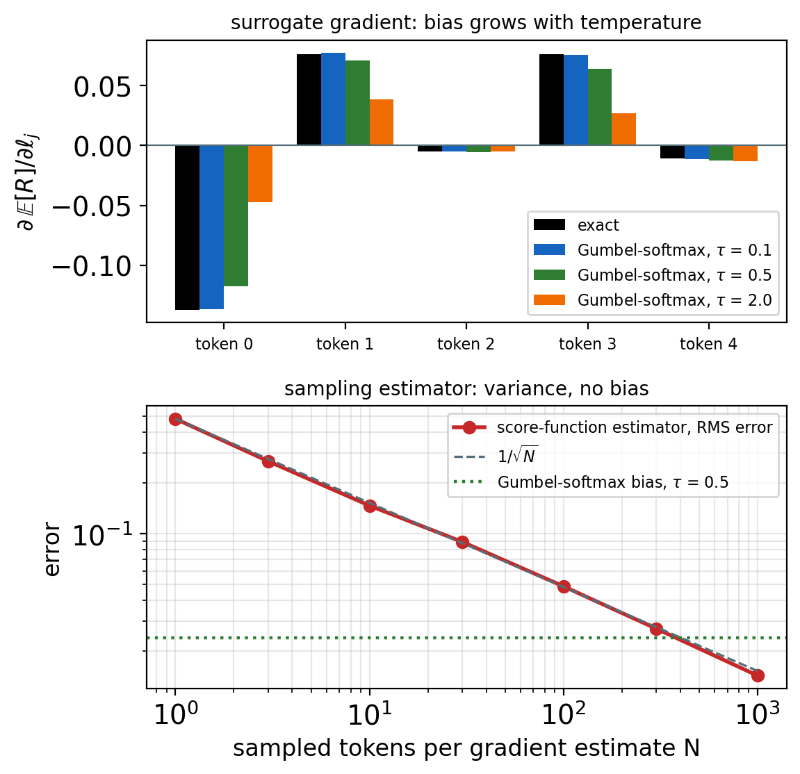
The same break appears wherever a categorical variable is sampled inside the graph - Gumbel-softmax is the categorical counterpart of reparameterization.
Each Family Trains Against a Different Divergence
Energy-based, maximum likelihood
- \(\text{KL}(p_{\text{data}} \,\|\, p_{\boldsymbol{\theta}})\), forward - every data mode must be covered, at any cost in spread
- Price: the negative phase, a sampling run inside every gradient
Variational autoencoder
- The same forward KL, minus the posterior gap - a bound, tight only where \(q\) matches the posterior
- Price: the gap, and averaged outputs wherever one mean must stand for several answers
Adversarial
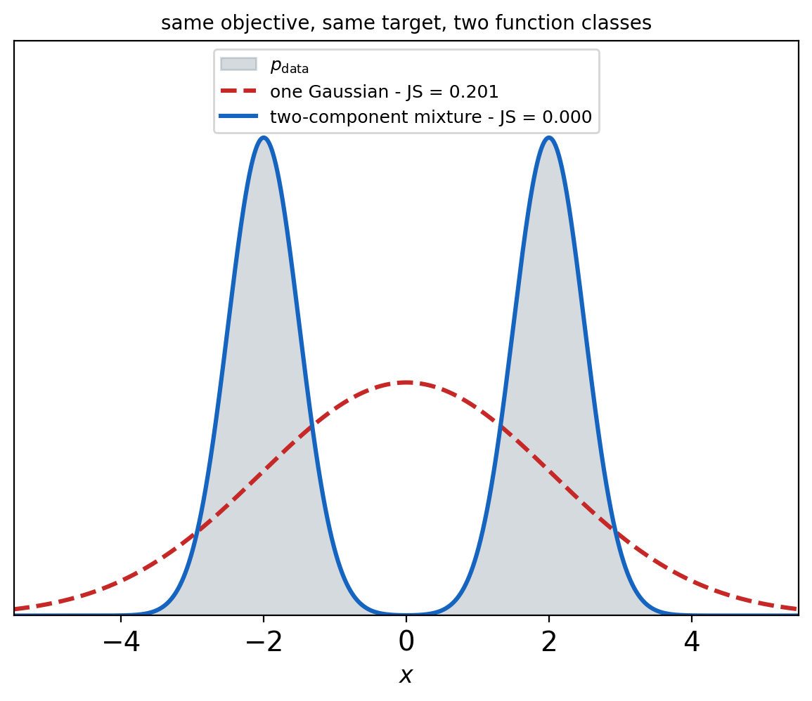
- At optimal \(D\): Jensen-Shannon - bounded, symmetric, and flat once the two distributions stop overlapping
- In practice, with the non-saturating loss: reverse-KL behavior - sharp samples, dropped modes tolerated
One model family, three objectives
- Forward KL covers both modes at every separation, reverse KL sits on one at every separation
- Jensen-Shannon covers when the modes are close and drops one when they are far - a bounded divergence pays at most \(\log 2\) for the drop, and covering keeps costing more as the gap grows
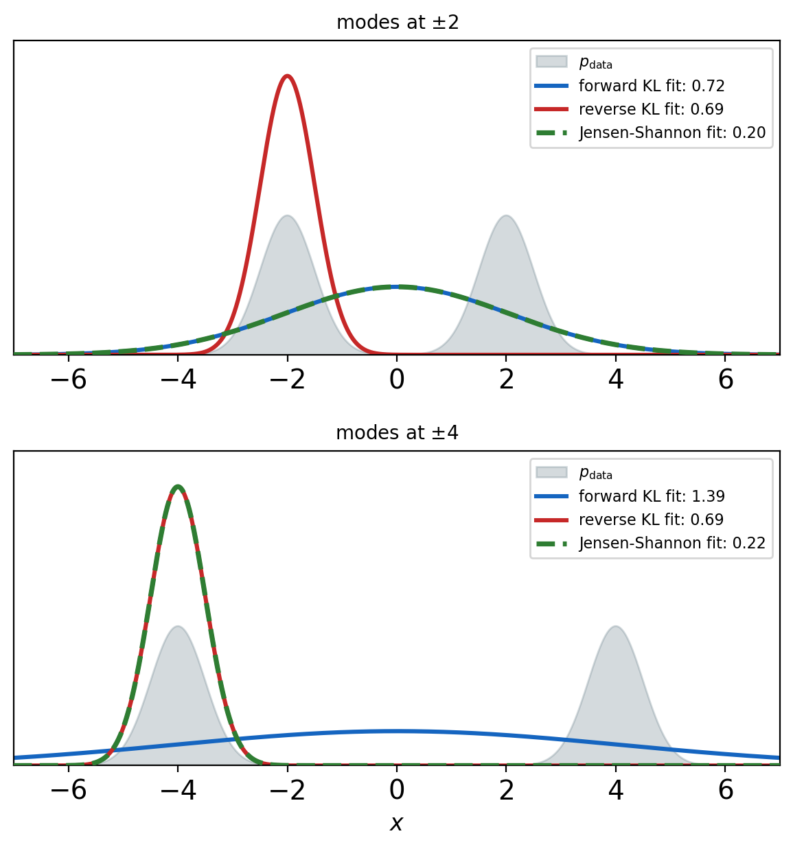
The errors a model makes are set by the divergence its training minimizes - the architecture decides only how well it can minimize it.
Diffusion Combines the Score and the Bound
Two lines meet
- Score matching across noise levels, from the energy-based family - a learned \(\nabla_{\mathbf{x}} \log p_\sigma(\mathbf{x})\) at every \(\sigma\), no partition function, no chain during training
- A hierarchical variational autoencoder with the encoder fixed to added noise - the same objective written as a lower bound, one KL term per noise level
- Sampling: Langevin steps on the learned score at decreasing noise - the chain returns, at generation time only
Sampling cost returns
- One sample costs \(T\) network passes, \(T\) in the hundreds to thousands - against one pass for a generator or a decoder
- Distillation to a few steps is where the adversarial loss survives - the discriminator as a training signal for a fast sampler
Codes as tokens
- A code-book index per position, from the VQ-VAE, and a learned model over the index grid - the bridge from images to models over token sequences
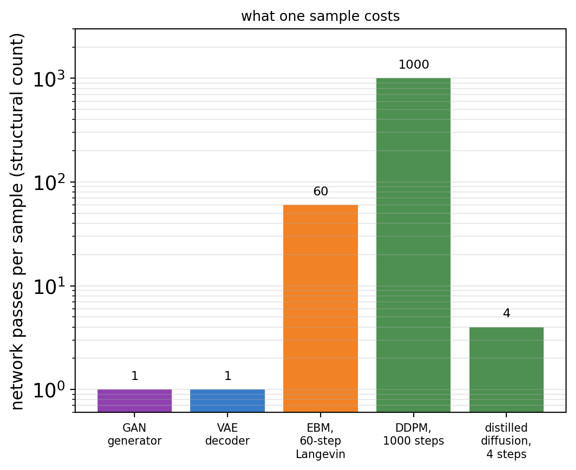
The families did not converge on a winner - the score, the bound, the code-book, and the discriminator each survive as a component of the models that followed.