Recurrent Neural Networks and Sequence-to-Sequence Models
EE 641 - Unit 4
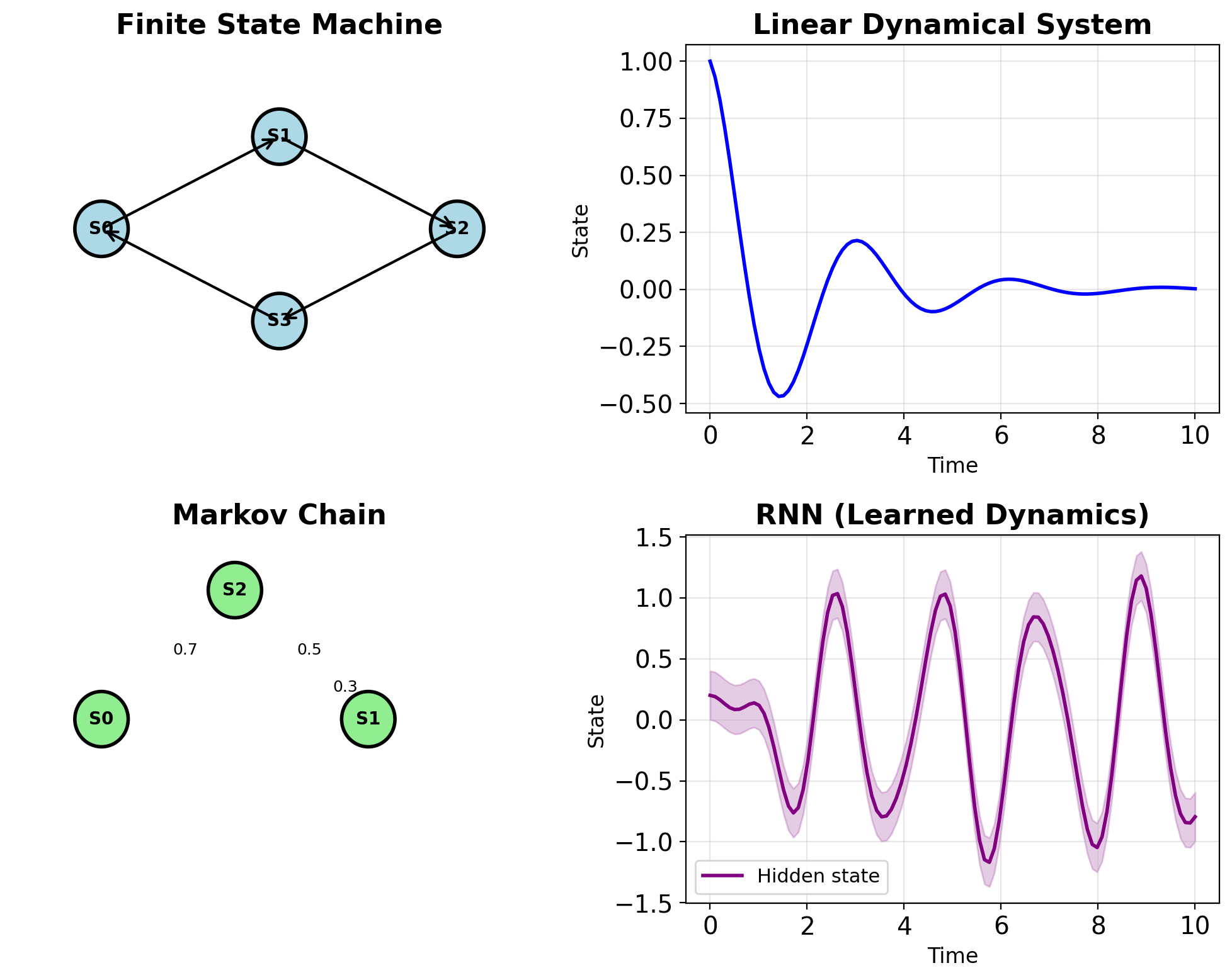
State Machine Complexity Hierarchy
| Type | State Space | Dynamics |
|---|---|---|
| FSM | Discrete, finite | Designed |
| Markov Chain | Discrete | Stochastic |
| Linear System | Continuous | Linear, fixed |
| Nonlinear System | Continuous | Nonlinear, fixed |
| RNN | Continuous | Nonlinear, learned |
RNNs optimize dynamics from data
- FSM: Hand-designed state transitions
- Linear system: Physics-based equations
- RNN: Gradient-based optimization
Recurrent and Unrolled Representations Are Mathematically Equivalent
Recurrent form (compact):
- Single state update block
- Feedback connection
- Direct implementation mapping
Unrolled form (explicit):
- Time as spatial dimension
- Each timestep = layer
- Explicit gradient computation
Mathematical equivalence: \[\mathbf{s}_t = f(\mathbf{s}_{t-1}, \mathbf{x}_t) = f(f(\mathbf{s}_{t-2}, \mathbf{x}_{t-1}), \mathbf{x}_t)\]
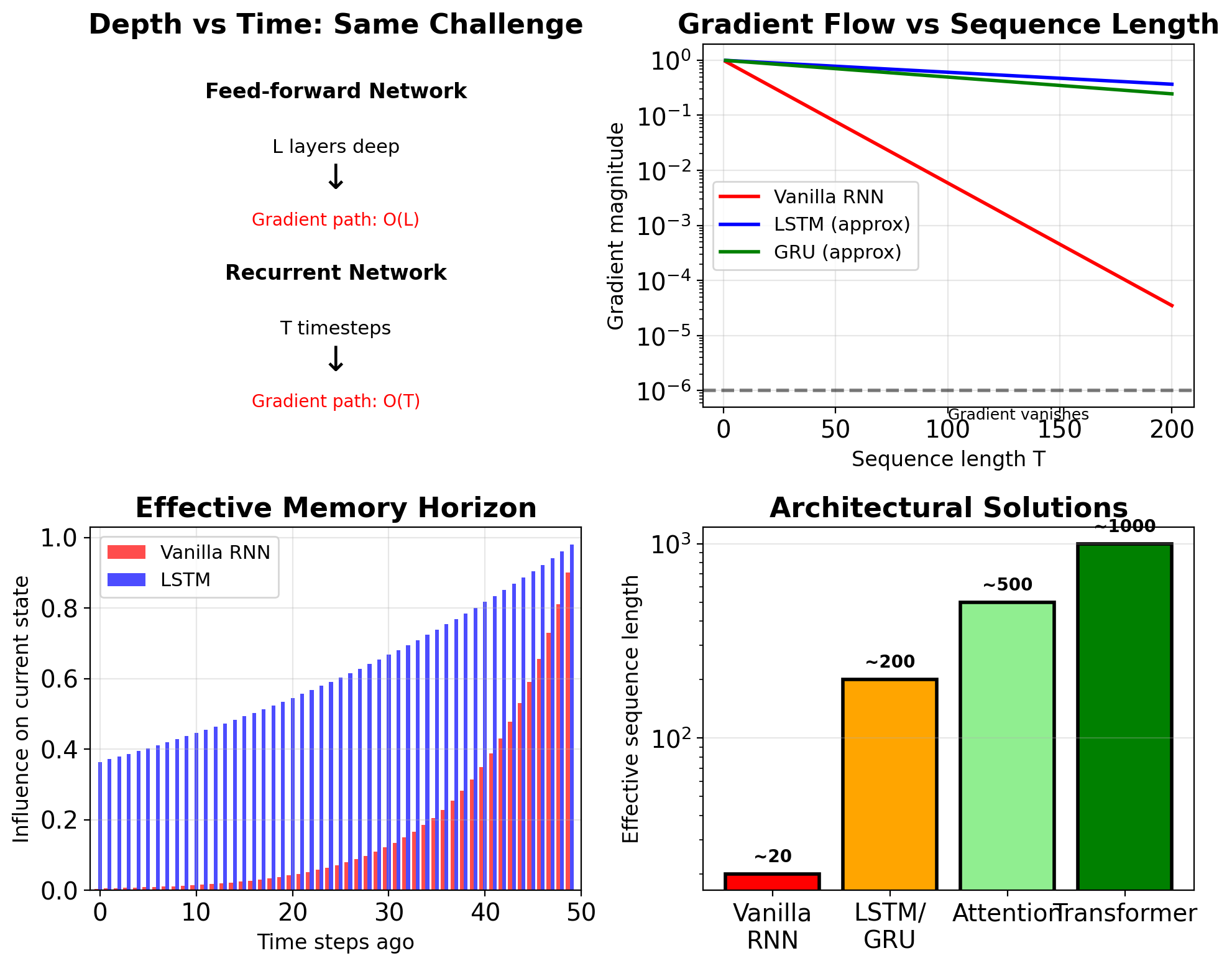
Unrolling depth = sequence length \(T\)
- Gradient path length: \(O(T)\)
- Memory requirement: \(O(T \times H)\)

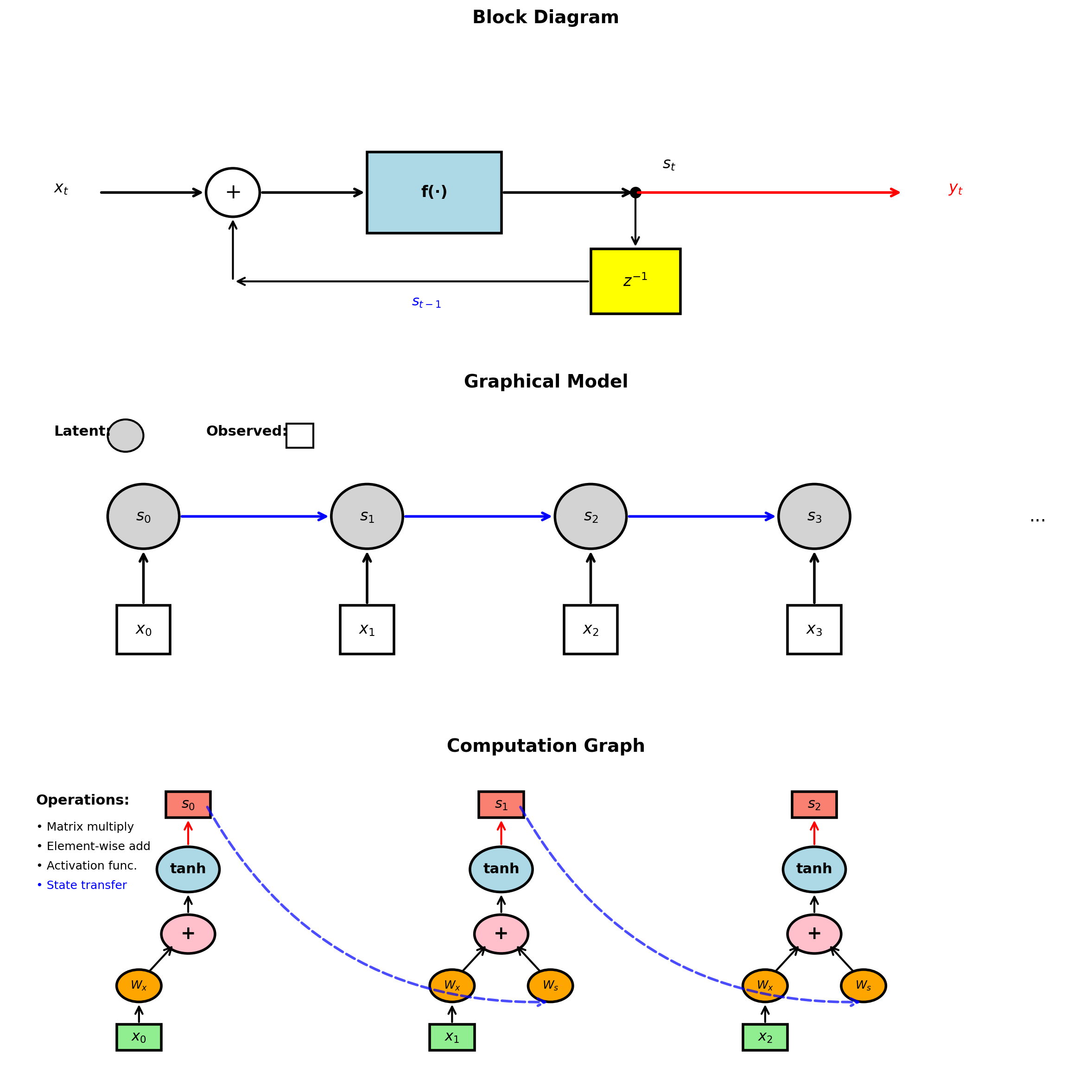
Multiple Representations of RNNs
Block diagram (Controls/DSP):
- Emphasizes signal flow
- Shows delay elements explicitly
- Standard in filter design
Graphical model (ML):
- Emphasizes dependencies
- Probabilistic interpretation
- Probabilistic inference ready
Computation graph (Deep Learning):
- Emphasizes operations
- Shows gradient flow
- Automatic differentiation compatible
All represent the same mathematics.
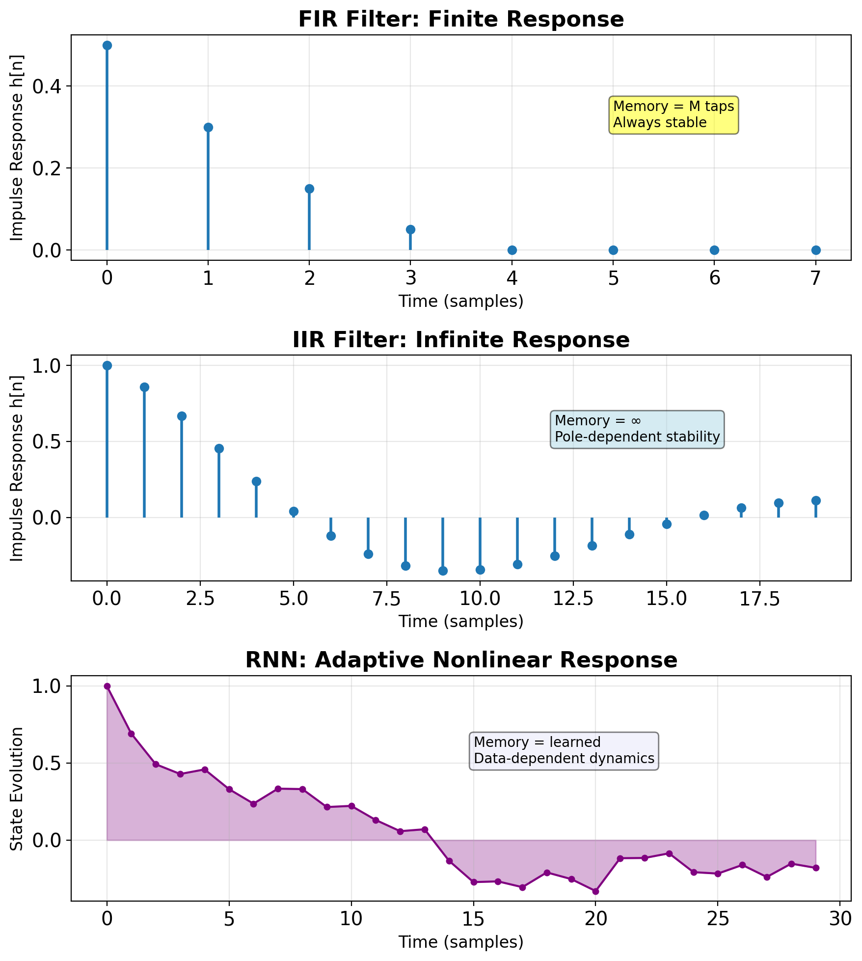
RNNs as Adaptive Nonlinear Filters
| Aspect | FIR Filter | IIR Filter | RNN |
|---|---|---|---|
| Response | Finite | Infinite | Infinite |
| Memory | Explicit (taps) | Implicit (poles) | Implicit (state) |
| Stability | Always stable | Depends on poles | Learned stability |
| Adaptation | LMS/RLS | Adaptive IIR | Backpropagation |
| Nonlinearity | None | None | Activation functions |
Signal processing interpretation:
- Hidden state = filter state variables
- Weights = filter coefficients
- Activation = nonlinear transfer function
- Training = adaptive filter optimization
RNNs: nonlinear adaptive filters in high-dimensional spaces
Discrete-Time Linear State-Space Systems
State update: \[\mathbf{s}_t = \mathbf{A}\mathbf{s}_{t-1} + \mathbf{B}\mathbf{u}_t\]
Output: \[\mathbf{y}_t = \mathbf{C}\mathbf{s}_t + \mathbf{D}\mathbf{u}_t\]
where:
- \(\mathbf{s}_t \in \mathbb{R}^n\) : state vector
- \(\mathbf{u}_t \in \mathbb{R}^m\) : input vector
- \(\mathbf{y}_t \in \mathbb{R}^p\) : output vector
- \(\mathbf{A} \in \mathbb{R}^{n \times n}\) : state transition matrix
- \(\mathbf{B} \in \mathbb{R}^{n \times m}\) : input matrix
- \(\mathbf{C} \in \mathbb{R}^{p \times n}\) : output matrix
Linearity enables closed-form analysis

Recursive Unrolling of State Evolution
Starting from \(\mathbf{s}_0\): \[\mathbf{s}_1 = \mathbf{A}\mathbf{s}_0 + \mathbf{B}\mathbf{u}_1\] \[\mathbf{s}_2 = \mathbf{A}\mathbf{s}_1 + \mathbf{B}\mathbf{u}_2 = \mathbf{A}^2\mathbf{s}_0 + \mathbf{A}\mathbf{B}\mathbf{u}_1 + \mathbf{B}\mathbf{u}_2\]
General solution: \[\mathbf{s}_t = \mathbf{A}^t\mathbf{s}_0 + \sum_{i=0}^{t-1}\mathbf{A}^i\mathbf{B}\mathbf{u}_{t-i}\]
Two components:
- Homogeneous: \(\mathbf{A}^t\mathbf{s}_0\) (initial condition response)
- Particular: \(\sum_{i=0}^{t-1}\mathbf{A}^i\mathbf{B}\mathbf{u}_{t-i}\) (input response)
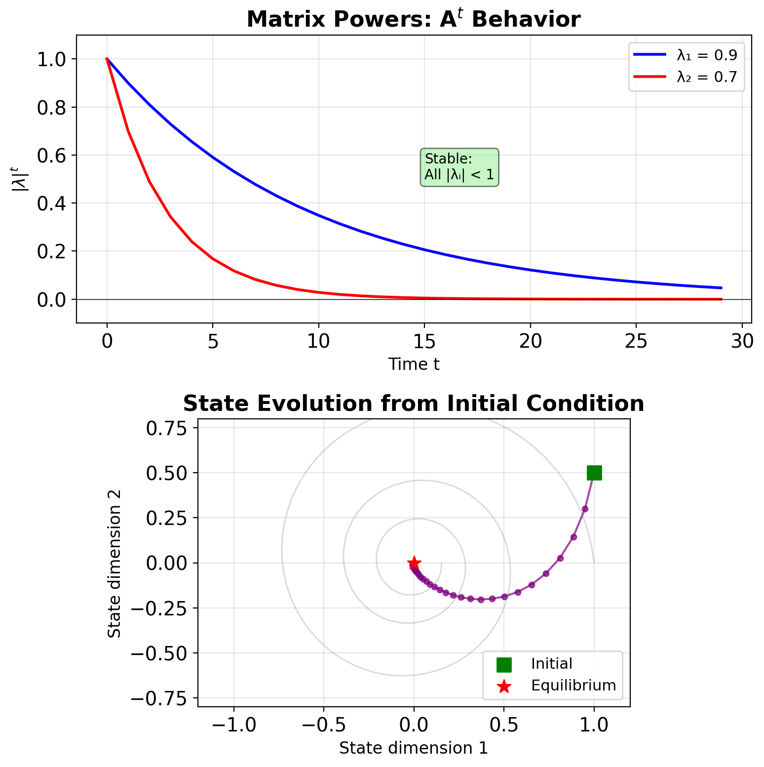
Long-term behavior dominated by \(\mathbf{A}^t\)
Diagonalization of System Dynamics
For diagonalizable \(\mathbf{A}\): \[\mathbf{A} = \mathbf{V}\boldsymbol{\Lambda}\mathbf{V}^{-1}\]
where:
- \(\mathbf{V} = [\mathbf{v}_1, ..., \mathbf{v}_n]\) : eigenvectors
- \(\boldsymbol{\Lambda} = \text{diag}(\lambda_1, ..., \lambda_n)\) : eigenvalues
Powers simplify: \[\mathbf{A}^t = \mathbf{V}\boldsymbol{\Lambda}^t\mathbf{V}^{-1}\] \[\boldsymbol{\Lambda}^t = \text{diag}(\lambda_1^t, ..., \lambda_n^t)\]
Eigenspace interpretation:
- Transform to eigenspace: \(\tilde{\mathbf{s}} = \mathbf{V}^{-1}\mathbf{s}\)
- Evolution: \(\tilde{s}_i(t) = \lambda_i^t \tilde{s}_i(0)\)
- Each mode evolves independently
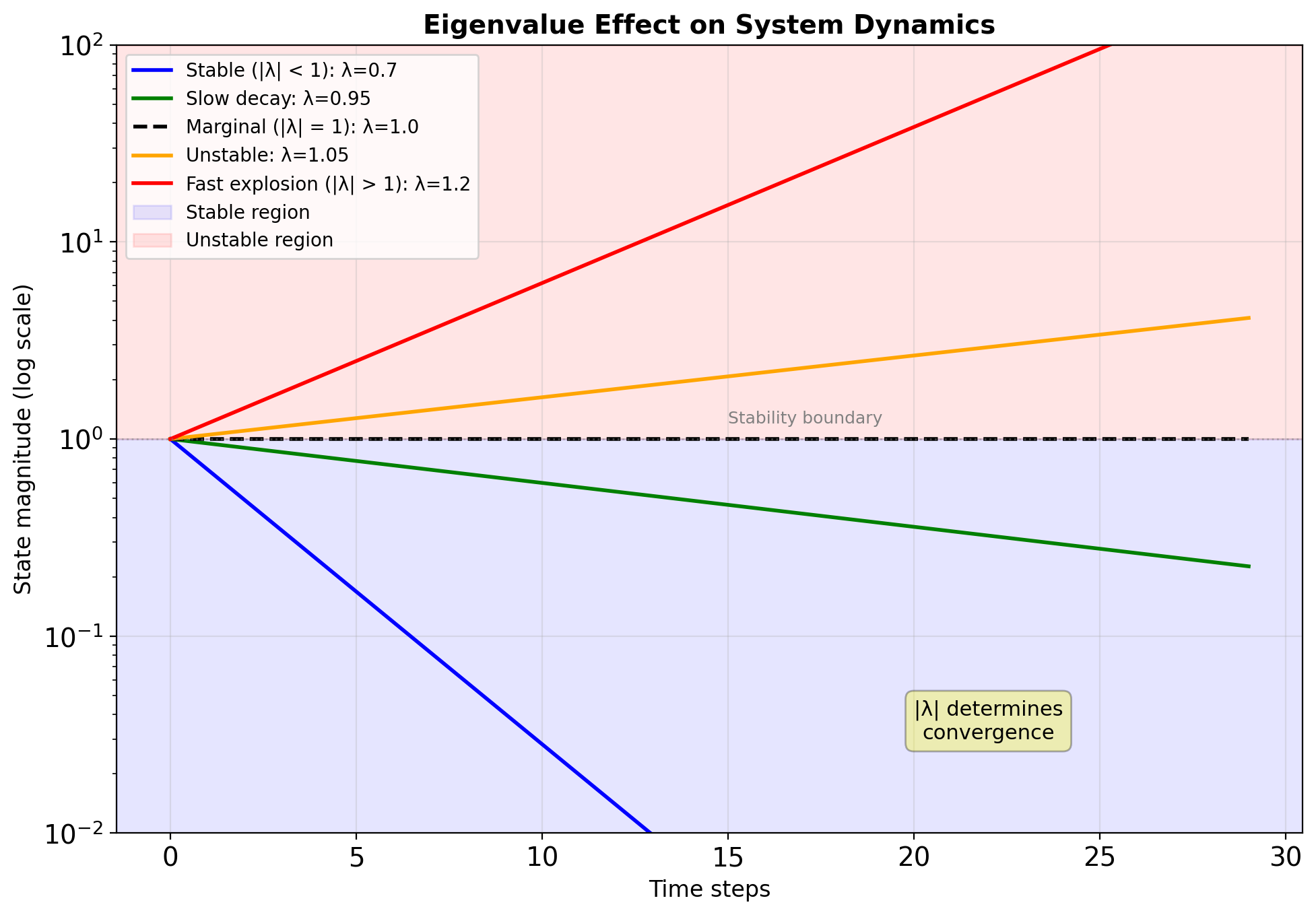
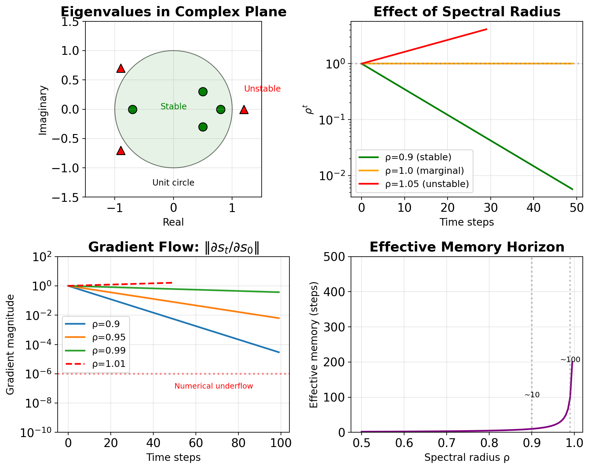
Spectral Radius Determines System Fate
\[\rho(\mathbf{A}) = \max_i |\lambda_i|\]
Stability conditions:
| Spectral Radius | Behavior | Gradient Flow |
|---|---|---|
| \(\rho < 1\) | Stable, converges to 0 | Vanishing |
| \(\rho = 1\) | Marginal stability | Preserved |
| \(\rho > 1\) | Unstable, diverges | Exploding |
For RNNs:
- Initialization: Often set \(\rho(\mathbf{W}_{ss}) \approx 1\)
- Training: Can drift from initialization
- Gradient flow: \(\|\frac{\partial \mathbf{s}_t}{\partial \mathbf{s}_0}\| \approx \rho^t\)
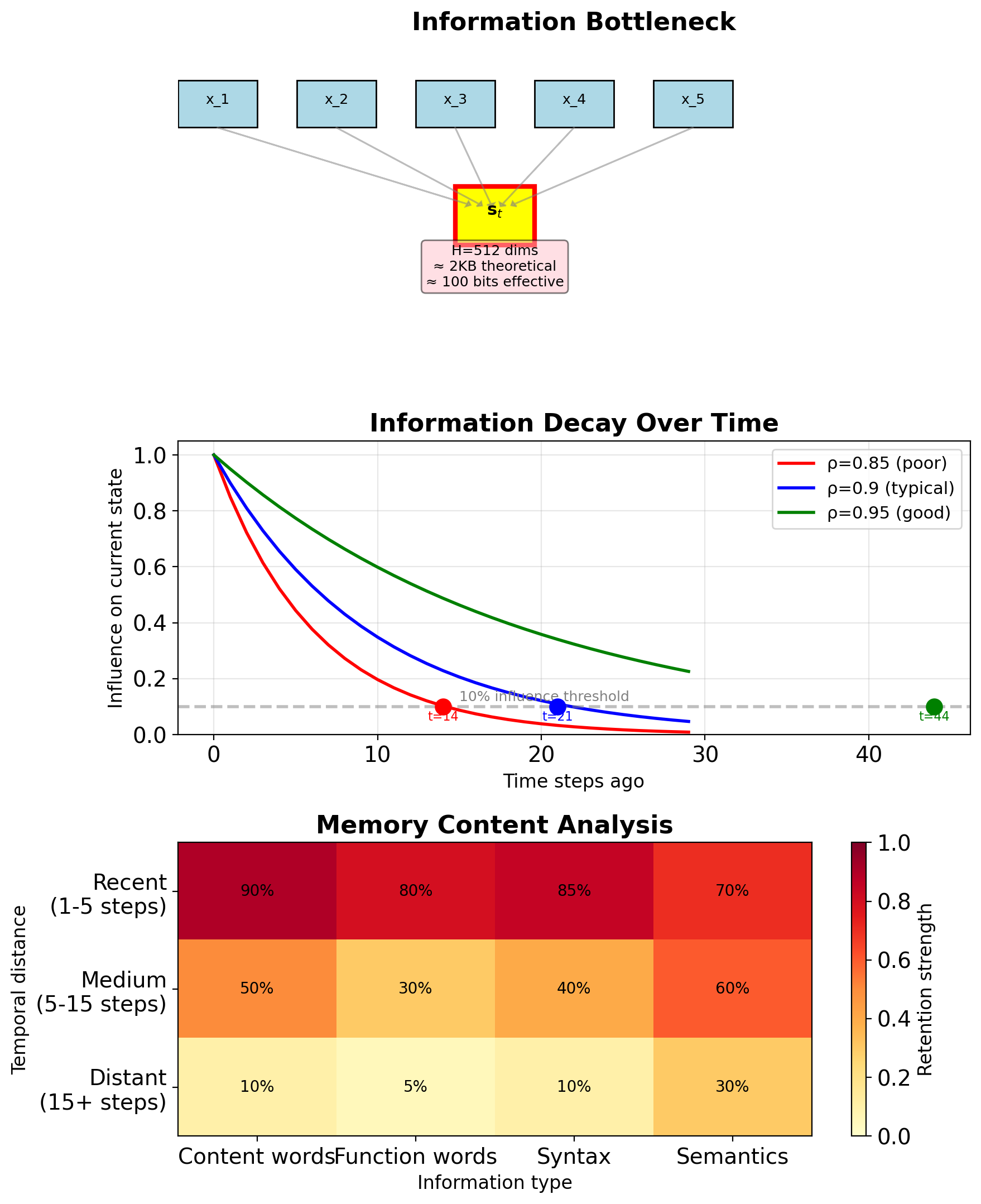
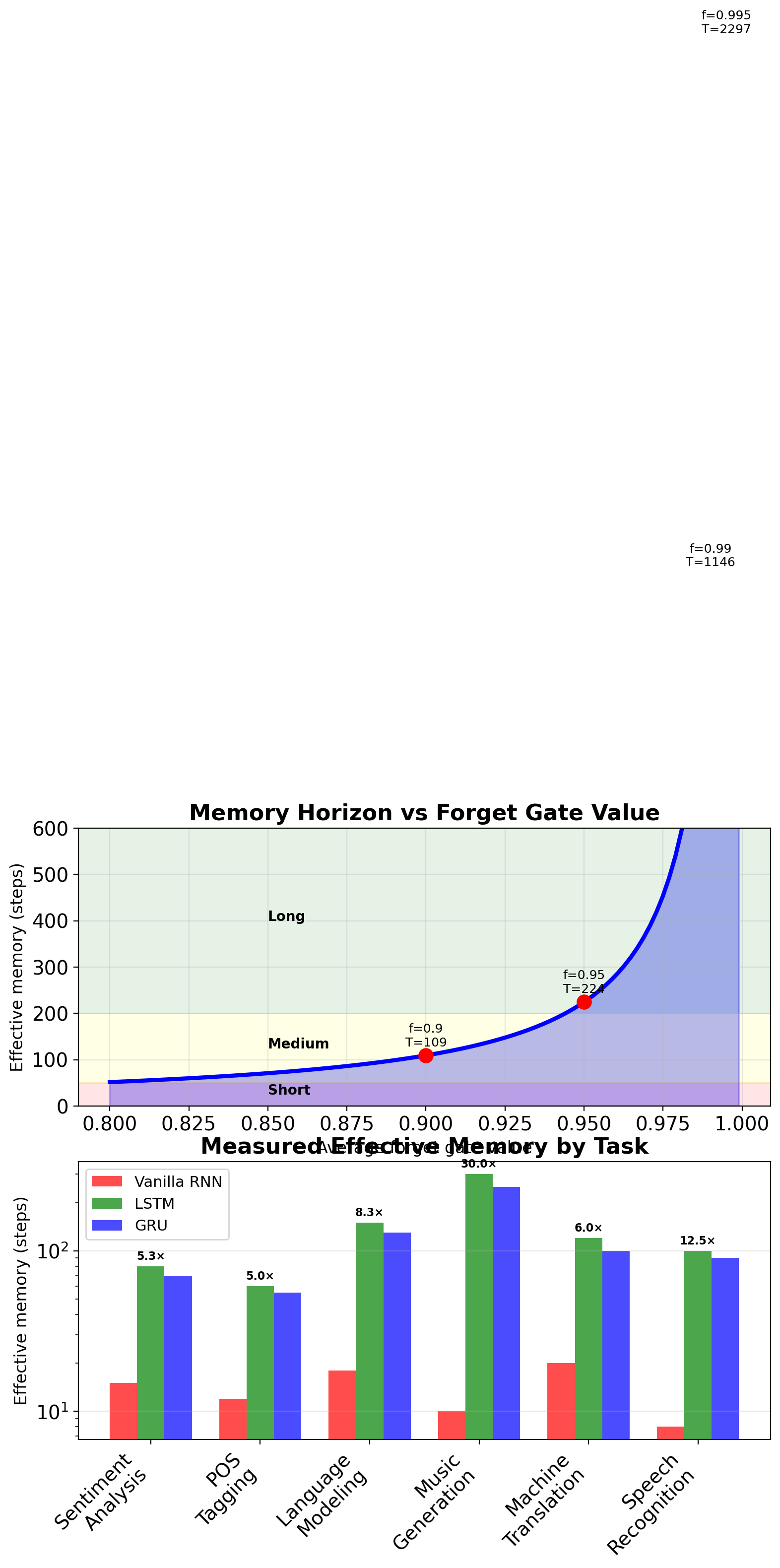
Time horizon: Effective memory \(\approx \frac{1}{1-\rho}\)
- \(\rho = 0.9\): ~10 steps
- \(\rho = 0.99\): ~100 steps
- \(\rho = 0.999\): ~1000 steps
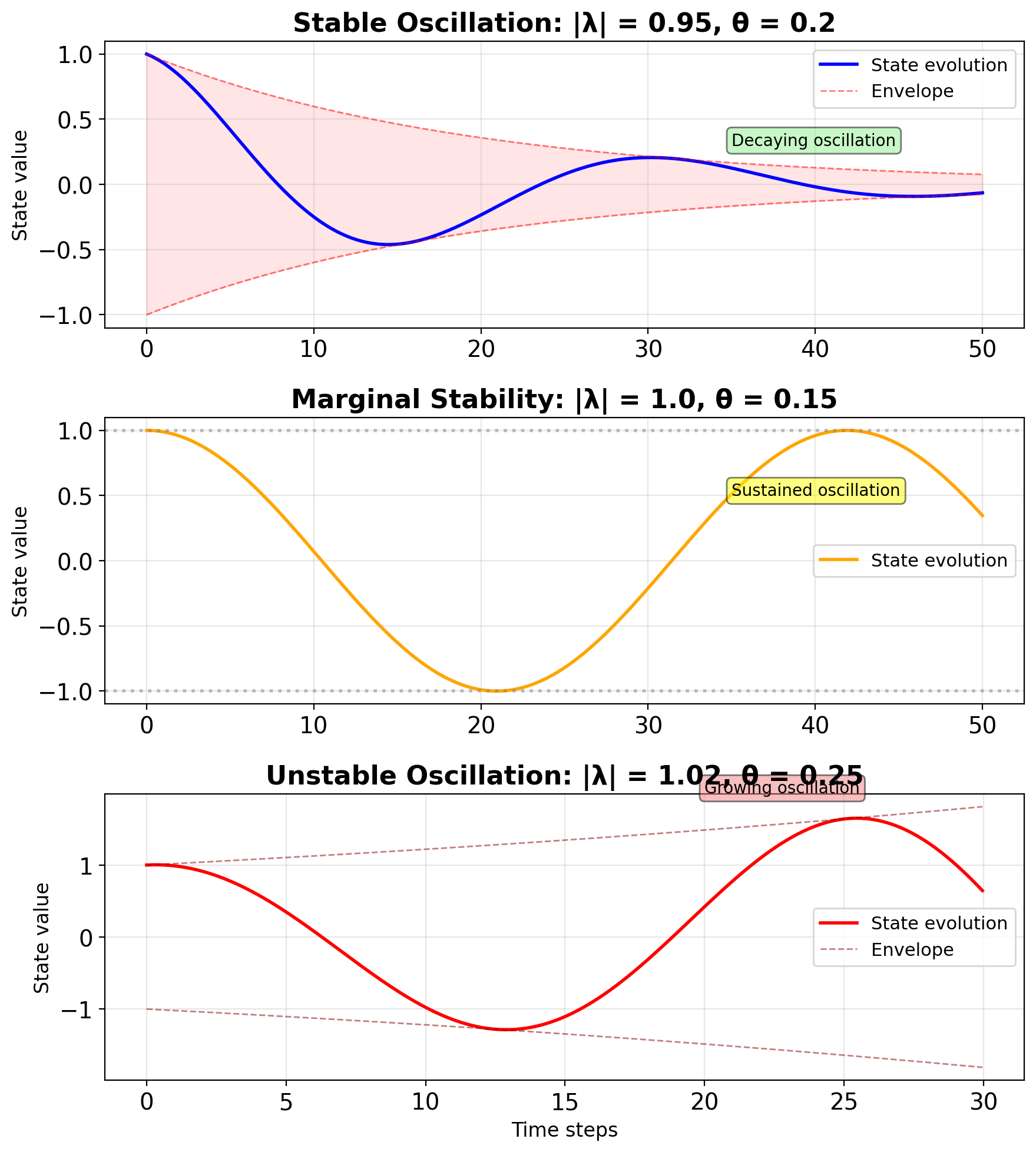
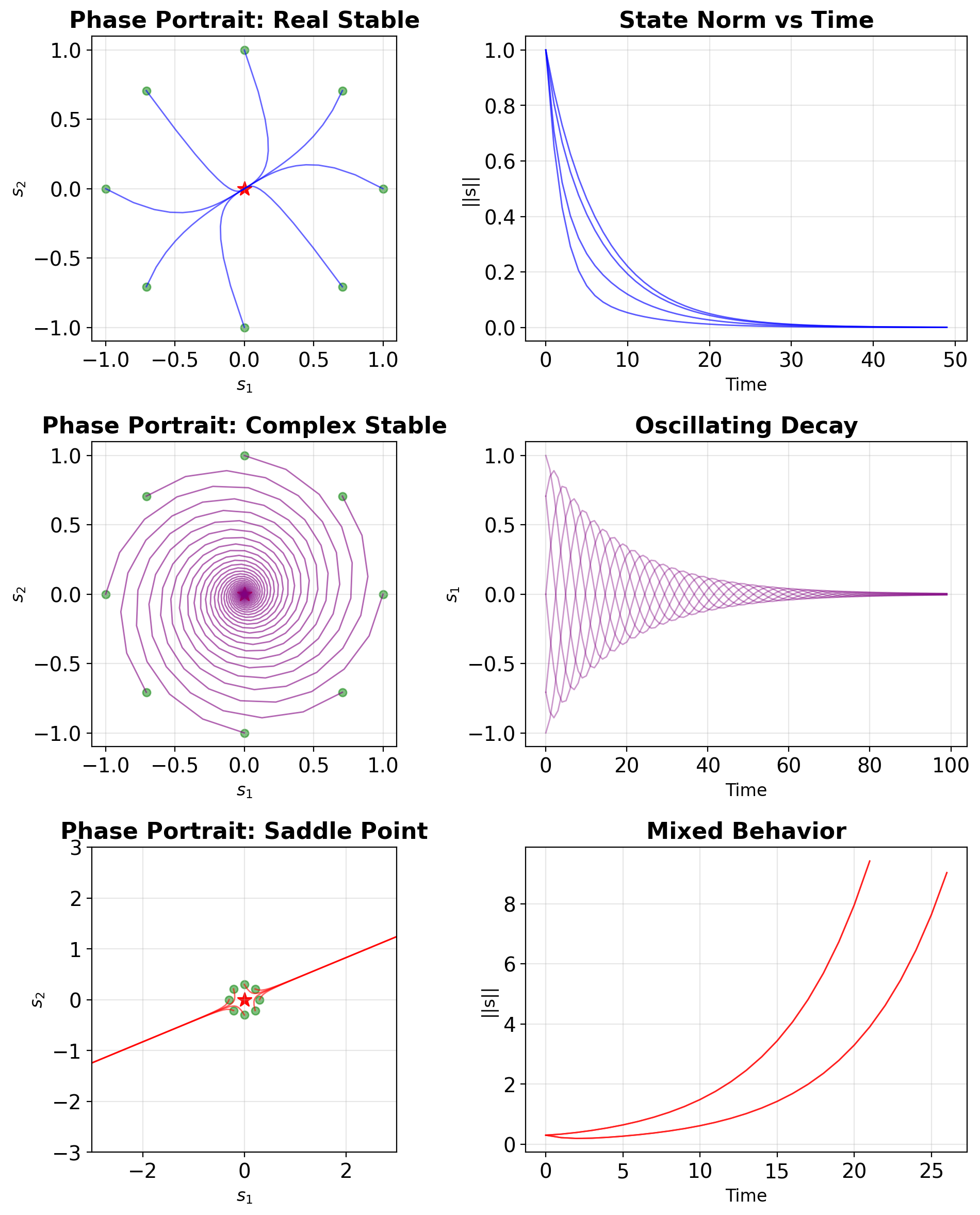
Complex Eigenvalues Create Oscillations
For real matrix \(\mathbf{A}\): \[\lambda = a \pm bi\]
Polar form: \[\lambda = r e^{\pm i\theta}\] where:
- \(r = |\lambda| = \sqrt{a^2 + b^2}\) : magnitude
- \(\theta = \arctan(b/a)\) : frequency
Evolution: \[\lambda^t = r^t e^{\pm it\theta} = r^t(\cos(t\theta) \pm i\sin(t\theta))\]
Results in:
- Exponential envelope: \(r^t\)
- Oscillation: \(\cos(t\theta)\), \(\sin(t\theta)\)
- Period: \(T = 2\pi/\theta\)
Three Characteristic 2×2 Cases
Case 1: Real, stable \[\mathbf{A}_1 = \begin{bmatrix} 0.8 & 0.1 \\ 0.1 & 0.7 \end{bmatrix}\] \(\lambda = \{0.9, 0.6\}\) → Monotonic decay
Case 2: Complex, stable \[\mathbf{A}_2 = \begin{bmatrix} 0.9 & 0.3 \\ -0.3 & 0.9 \end{bmatrix}\] \(\lambda = 0.9 \pm 0.3i\) → Decaying spiral
Case 3: Real, mixed \[\mathbf{A}_3 = \begin{bmatrix} 1.1 & 0.2 \\ 0.2 & 0.7 \end{bmatrix}\] \(\lambda = \{1.2, 0.6\}\) → Saddle point
Each case has distinct implications for gradient flow in RNNs
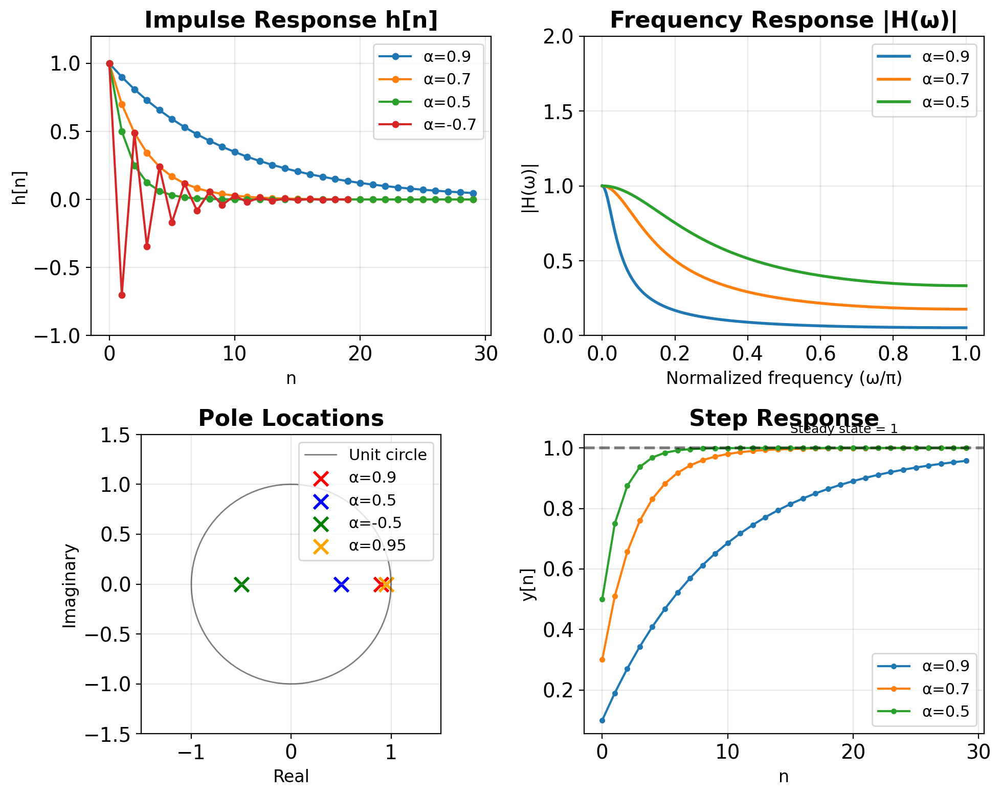
First-Order AR Filter Review
First-order AR filter: \[y[n] = \alpha y[n-1] + \beta x[n]\]
Transfer function: \[H(z) = \frac{\beta}{1 - \alpha z^{-1}}\]
Pole location determines behavior:
- \(|\alpha| < 1\) : Stable (pole inside unit circle)
- \(0 < \alpha < 1\) : Low-pass characteristic
- \(-1 < \alpha < 0\) : Oscillatory response
- \(|\alpha| \geq 1\) : Unstable
DC gain (steady-state response): \[H(1) = \frac{\beta}{1 - \alpha}\]
For unit DC gain: \(\beta = 1 - \alpha\)
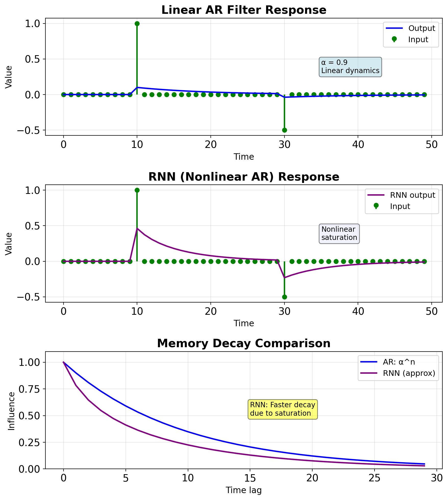
RNN as Nonlinear AR Filter
Linear AR (vector form): \[\mathbf{s}_t = \mathbf{A}\mathbf{s}_{t-1} + \mathbf{B}\mathbf{x}_t\]
Vanilla RNN: \[\mathbf{s}_t = \tanh(\mathbf{W}_{ss}\mathbf{s}_{t-1} + \mathbf{W}_{xs}\mathbf{x}_t + \mathbf{b})\]
Generalizations:
- Nonlinear activation (tanh) vs linear
- Learned coefficients vs designed
- High-dimensional state vs scalar/low-dim
- Data-adaptive vs fixed
Memory mechanism:
- AR filter: Exponential decay \(\alpha^n\)
- RNN: Complex, input-dependent decay
- Both: State provides implicit memory
Stability:
- AR: \(|\alpha| < 1\)
- RNN: \(\rho(\mathbf{W}_{ss}) \cdot |\tanh'| < 1\)
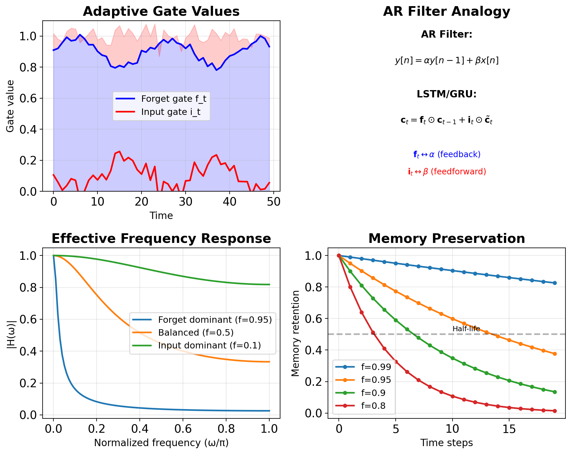
Filter Perspective on Gates
Forget gate (feedback coefficient): \[\mathbf{f}_t = \sigma(\mathbf{W}_f[\mathbf{s}_{t-1}, \mathbf{x}_t] + \mathbf{b}_f)\]
- Analogous to \(\alpha\) in AR filter
- Controls memory retention
- Learned per timestep and dimension
Input gate (feedforward coefficient): \[\mathbf{i}_t = \sigma(\mathbf{W}_i[\mathbf{s}_{t-1}, \mathbf{x}_t] + \mathbf{b}_i)\]
- Analogous to \(\beta\) in AR filter
- Controls new information integration
Coupled gates for unit DC gain:
- GRU: \(\mathbf{z}_t\) and \((1-\mathbf{z}_t)\)
- Ensures \(\mathbf{f}_t + \mathbf{i}_t \approx 1\)
- Preserves signal magnitude
Frequency Domain Intuition
Linear system frequency response:
- Fixed for all inputs
- Determined by poles/zeros
- Time-invariant filtering
RNN frequency response:
- Input-dependent through gates
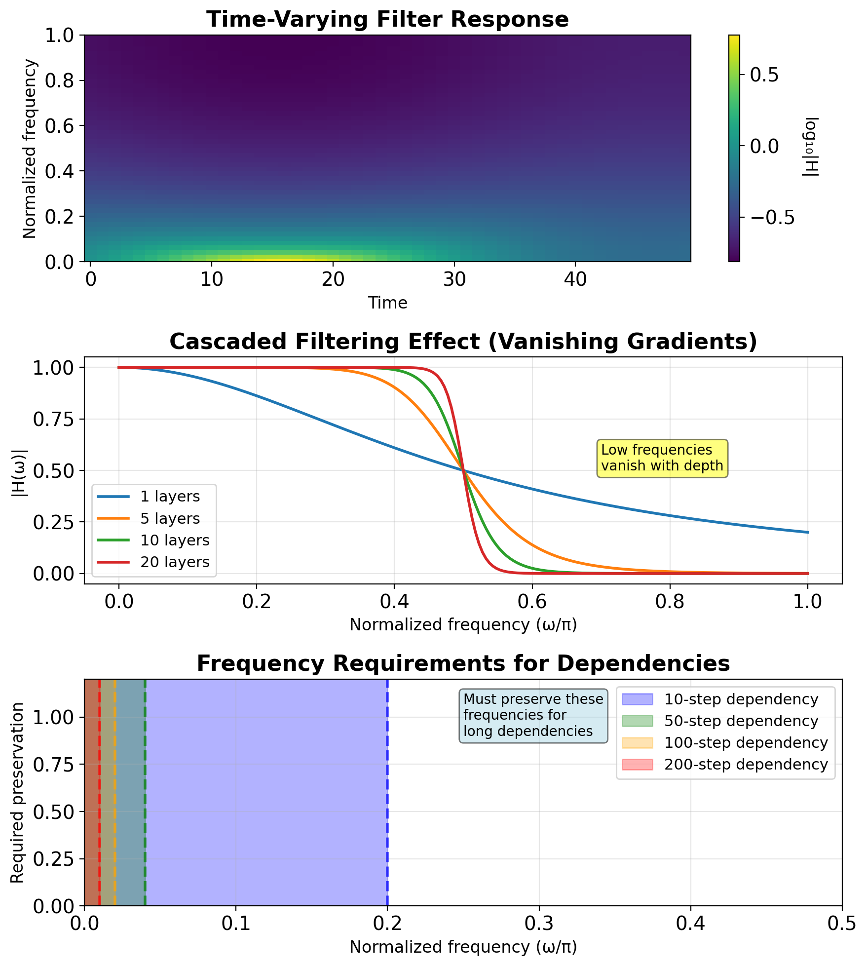
- Time-varying filter characteristics
- Adaptive bandwidth
Long-term dependencies = Low frequencies
- Need to preserve DC and low freq
- Forget gate ≈ 1 preserves low freq
Vanishing gradients = High-pass filtering
- Each tanh acts as low-pass
- Cascaded effect removes low freq
Gates modulate bandwidth
- High forget gate: Wider bandwidth
- Low forget gate: Narrow, input-focused
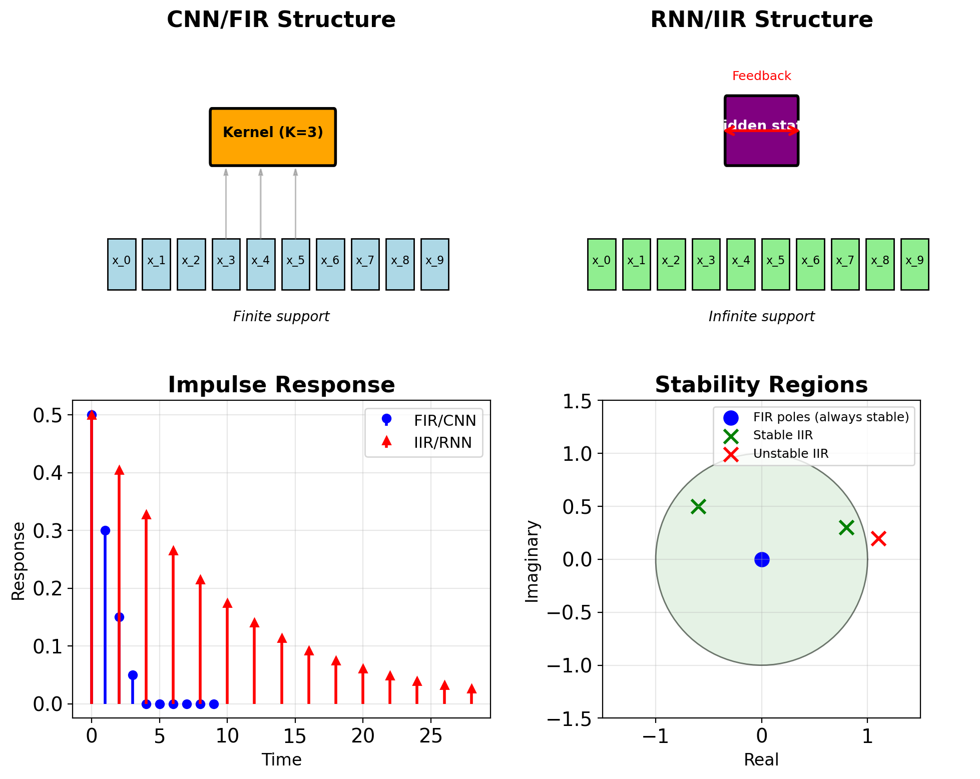
IIR vs FIR Analogy
CNNs = FIR Filters
- Finite receptive field (kernel size)
- No feedback connections
- Always stable
- Explicit memory (stored activations)
- Parallel computation possible
RNNs = IIR Filters
- Infinite receptive field (in principle)
- Feedback through hidden state
- Can be unstable
- Implicit memory (compressed state)
- Sequential computation required
Comparison:
- Memory: FIR needs O(K), IIR needs O(1)
- Computation: FIR is O(K) parallel, IIR is O(1) sequential
- Stability: FIR guaranteed, IIR conditional
- Design: FIR straightforward, IIR complex
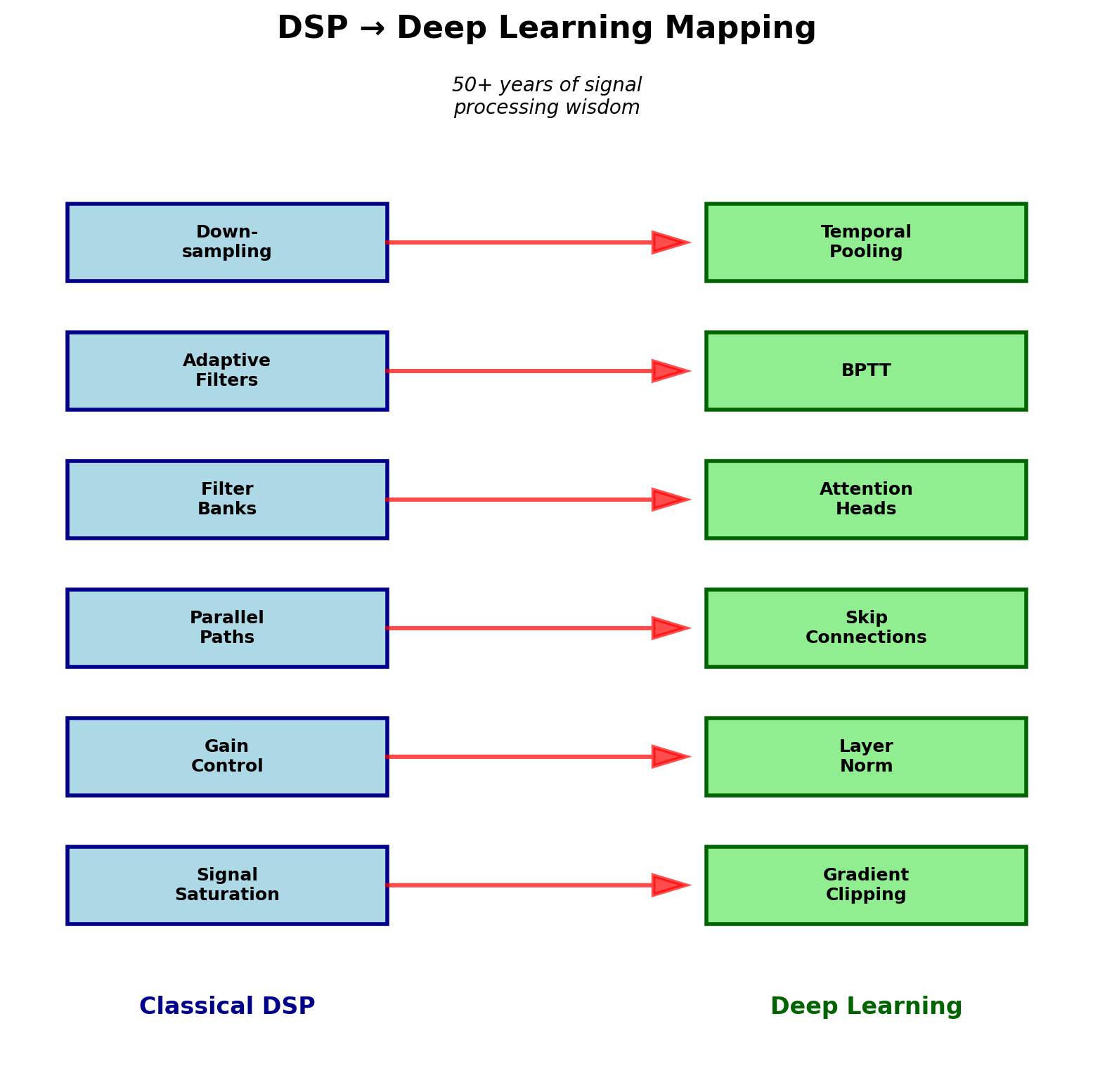
Signal Processing Insights
| DSP Concept | RNN Equivalent | Purpose |
|---|---|---|
| Saturation/Limiting | Gradient clipping | Prevent overflow |
| AGC | Layer norm | Stabilize magnitude |
| Parallel paths | Skip connections | Preserve signal |
| Filter bank | Attention heads | Frequency decomposition |
| Adaptive filtering | BPTT | Learn coefficients |
| Decimation | Pooling in time | Reduce rate |
| Interpolation | Upsampling | Increase rate |
- Many “tricks” in deep learning have DSP origins
- Signal flow analysis helps debug networks
- Frequency domain reveals failure modes
- Classical solutions inspire new architectures
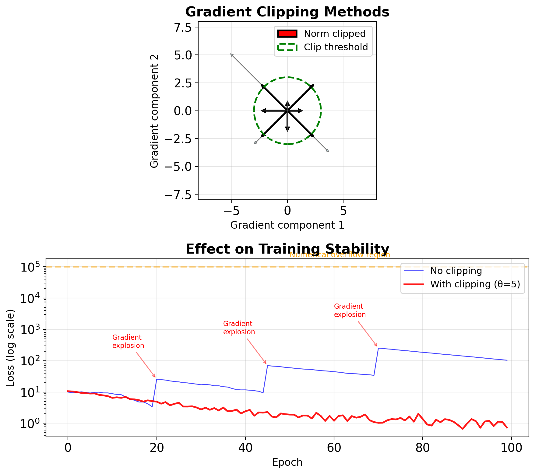
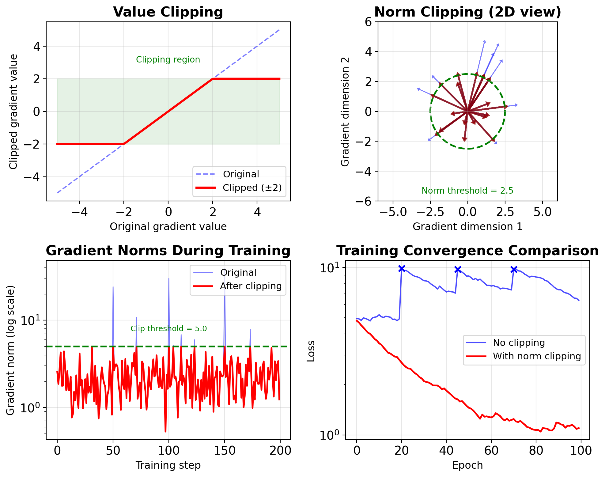
Gradient Clipping as Signal Saturation
Classical DSP: Saturation prevents amplifier damage
- Input exceeds linear range
- Output clipped to safe levels
- Prevents system damage
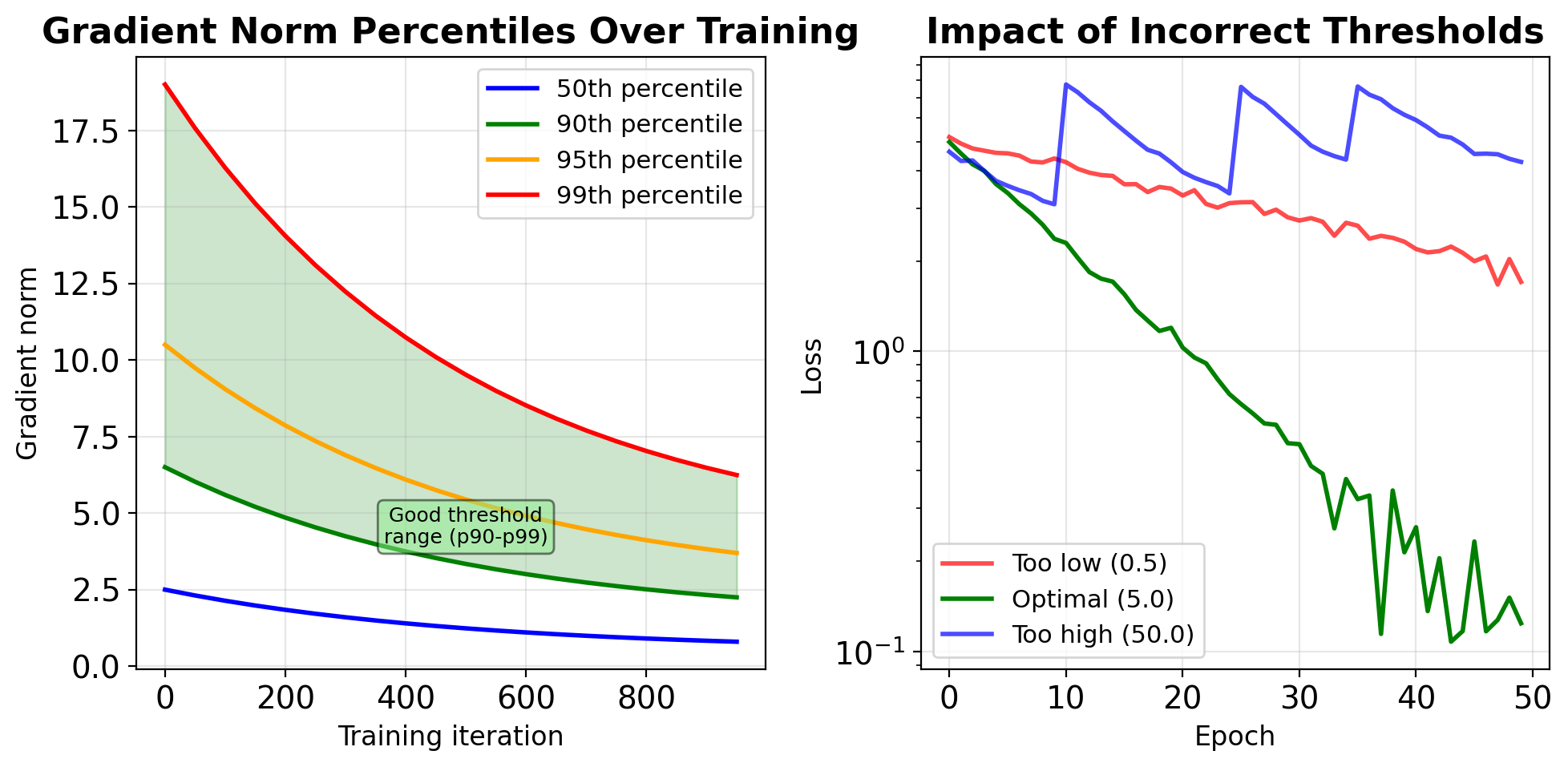
Deep Learning: Gradient clipping prevents training instability \[\mathbf{g}_{\text{clipped}} = \begin{cases} \mathbf{g} & \text{if } \|\mathbf{g}\| \leq \theta \\ \theta \cdot \frac{\mathbf{g}}{\|\mathbf{g}\|} & \text{if } \|\mathbf{g}\| > \theta \end{cases}\]
Two clipping strategies:
Value clipping: Element-wise bounds
- Simple but can change gradient direction
Norm clipping: Preserves direction
- Standard for RNNs (typical θ = 5-10)
Empirical thresholds (LSTM on PTB):
- No clipping: 38% training failures
- θ = 5: Stable, perplexity 78.4
- θ = 1: Over-constrained, perplexity 92.1
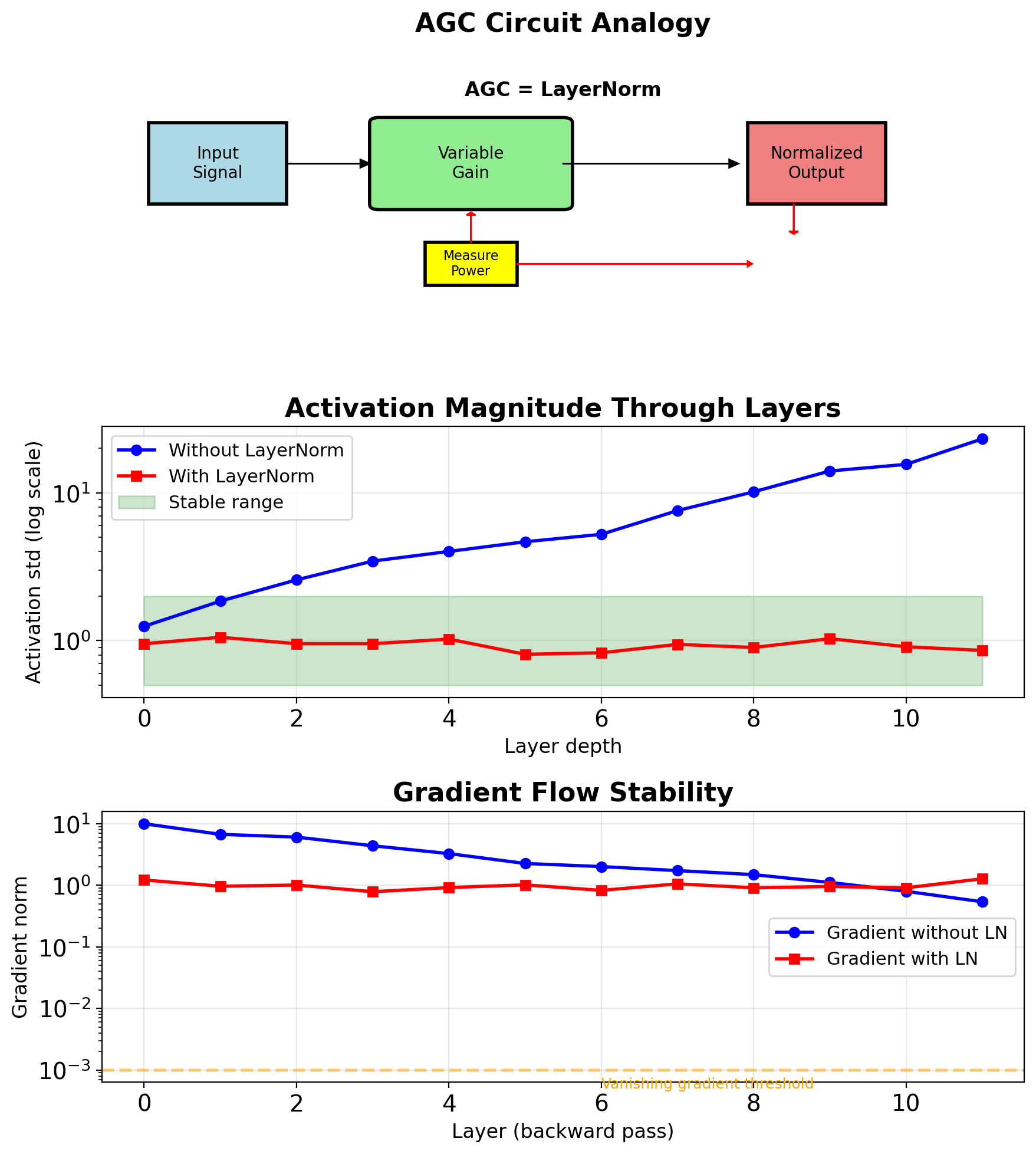
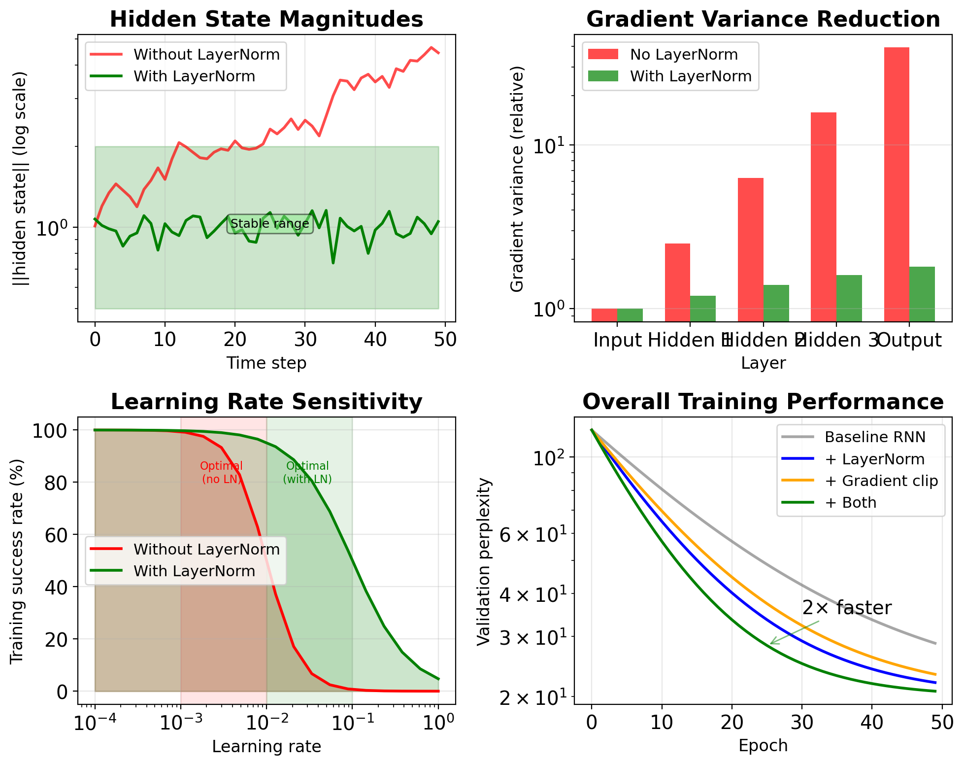
Layer Normalization as Automatic Gain Control
Classical AGC (Automatic Gain Control):
- Maintains constant output level
- Adapts to input signal variations
- Used in radio/audio systems
Layer Normalization: \[\text{LN}(\mathbf{x}) = \gamma \frac{\mathbf{x} - \mu}{\sqrt{\sigma^2 + \epsilon}} + \beta\]
where across feature dimension:
\(\mu = \frac{1}{D}\sum_{i=1}^D x_i\)
\(\sigma^2 = \frac{1}{D}\sum_{i=1}^D (x_i - \mu)^2\)
AGC: Normalizes signal power
LayerNorm: Normalizes activation magnitude
Both prevent saturation in subsequent stages
Measured stabilization (Transformer, 12 layers):
- Without LN: Activation std varies 10²-10⁴
- With LN: Activation std stays in [0.8, 1.2]
- Training speedup: 5.3×
Skip Connections as Parallel Signal Paths
DSP: Parallel signal paths
- Preserve different frequency bands
- Combine for complete signal
- Prevent information loss
ResNet skip connections: \[\mathbf{y} = F(\mathbf{x}, \mathbf{W}) + \mathbf{x}\]
Gradient flow analysis: \[\frac{\partial L}{\partial \mathbf{x}} = \frac{\partial L}{\partial \mathbf{y}} \left(1 + \frac{\partial F}{\partial \mathbf{x}}\right)\]
Even if \(\frac{\partial F}{\partial \mathbf{x}} \approx 0\) (vanishing), gradient still flows through identity path
Frequency domain interpretation:
- Main path: Learned transformation with possible attenuation
- Skip path: All-pass filter (preserves all frequencies)
- Combined: Guaranteed minimum gain of 1
Impact on trainability (ImageNet):
- 34-layer plain net: 28.5% error
- 34-layer ResNet: 25.0% error
- 152-layer ResNet: 23.0% error (deeper is better!)

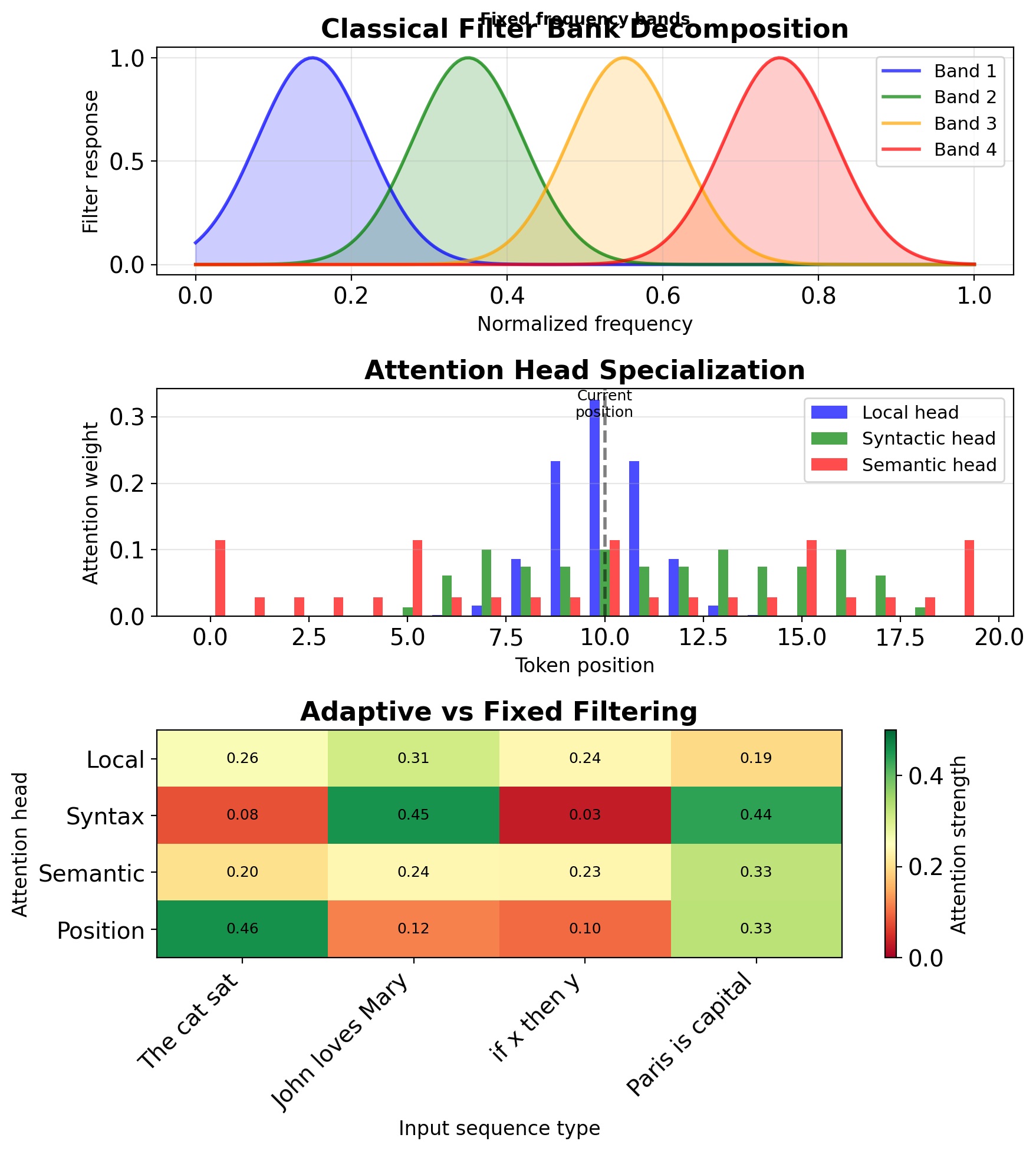
Attention as Adaptive Filter Banks
Filter banks in DSP vs attention mechanisms
Classical filter bank:
- Decompose signal into frequency bands
- Process each band separately
- Reconstruct from components
Multi-head attention as filter bank: \[\text{Attention}(Q,K,V) = \text{softmax}\left(\frac{QK^T}{\sqrt{d_k}}\right)V\]
Each head captures different “frequency” of relationships:
- Head 1: Local dependencies (high freq)
- Head 2: Syntactic patterns (mid freq)
- Head 3: Semantic relations (low freq)
Adaptive aspect:
- Classical: Fixed frequency bands
- Attention: Data-dependent filtering
- Learned decomposition per input
Measured specialization (BERT-base):
- Heads 1-3: Position encoding (avg distance 2.1 tokens)
- Heads 4-6: Syntax (avg distance 5.7 tokens)
- Heads 7-12: Semantics (avg distance 11.3 tokens)
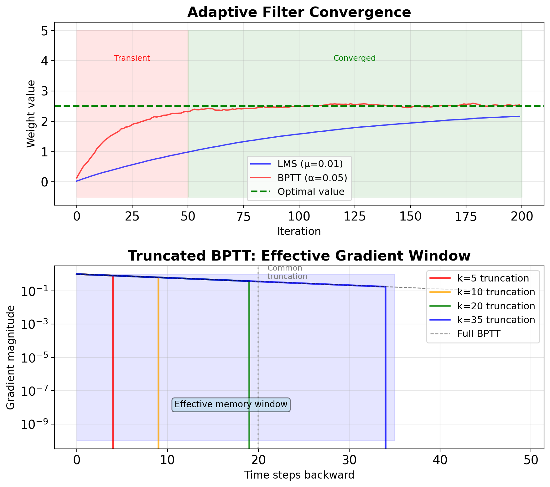
Adaptive Filtering and BPTT
Adaptive filters learn optimal coefficients
Classical adaptive filtering (LMS, RLS):
- Online coefficient updates
- Minimize prediction error
- Converge to optimal filter
BPTT as adaptive filter training: \[\mathbf{W}_{t+1} = \mathbf{W}_t - \alpha \nabla_{\mathbf{W}} L\]
- LMS: \(w_{n+1} = w_n + \mu e_n x_n\)
- BPTT: \(W_{ij}^{(t+1)} = W_{ij}^{(t)} - \alpha \frac{\partial L}{\partial W_{ij}}\)
Both minimize prediction error through iterative updates
Convergence characteristics:
- LMS: \(O(1/\mu)\) iterations, local minima
- BPTT: Depends on sequence length T
- Both sensitive to learning rate/step size
Truncated BPTT = Finite impulse response:
- Limit gradient flow to k steps
- Trade accuracy for stability
- Standard k = 20-35 for RNNs
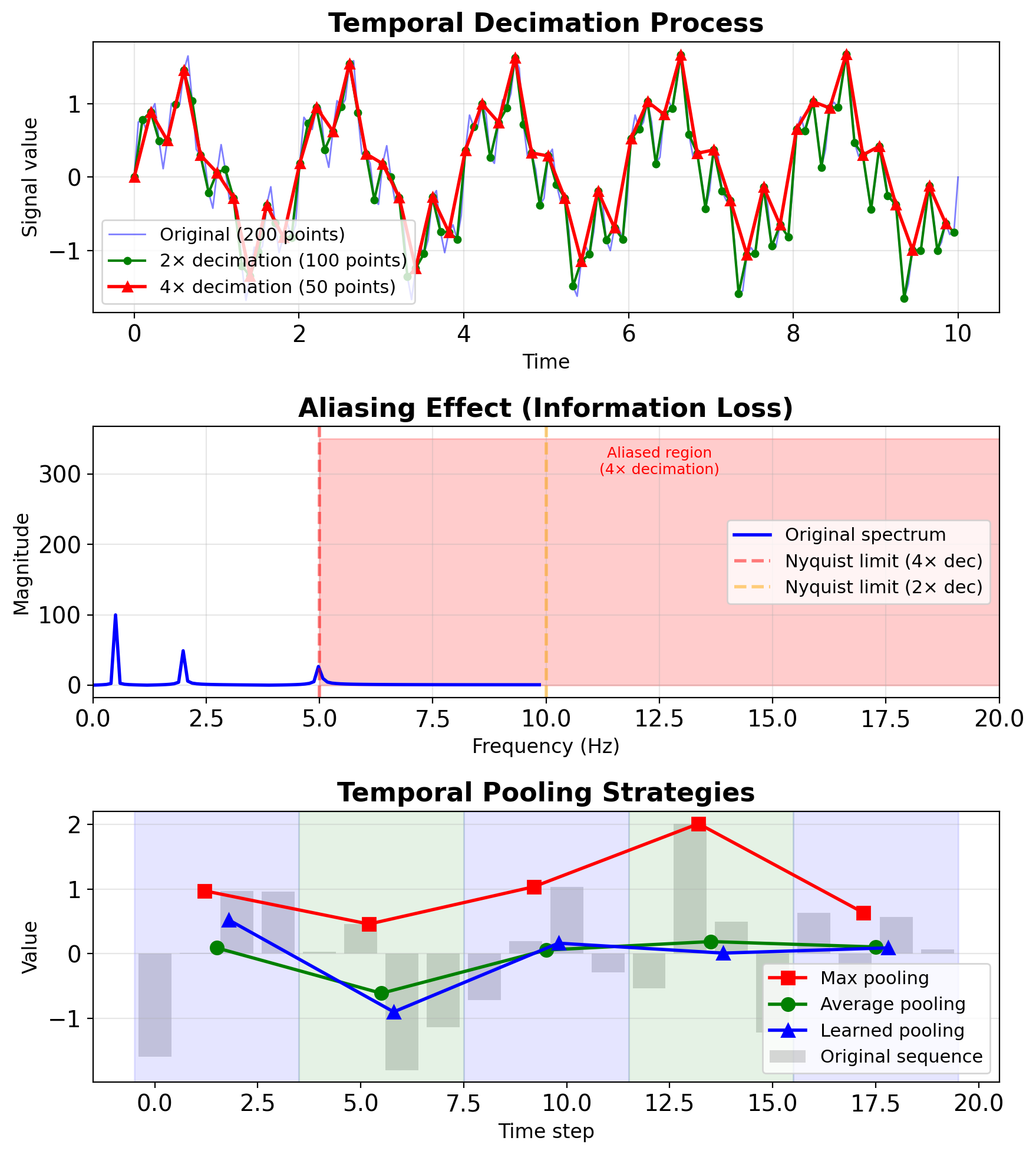
Temporal Decimation and Pooling
Decimation in DSP vs temporal pooling
DSP Decimation:
- Reduce sampling rate by factor M
- Must filter first (prevent aliasing)
- Nyquist criterion: \(f_s > 2f_{max}\)
Temporal pooling in RNNs:
- Reduce sequence length
- Aggregate temporal information
- Lower computational cost
Common strategies:
- Max pooling over time: Keep strongest signal
- Average pooling: Smooth temporal variations
- Strided convolutions: Learned decimation
Computational savings:
- Original: \(O(T \times d^2)\) per layer
- After 2× decimation: \(O(T/2 \times d^2)\)
- Memory reduction: 50%
Performance-memory (speech recognition):
- No pooling: 95.2% accuracy, 8GB memory
- 2× pooling: 94.8% accuracy, 4GB memory
- 4× pooling: 92.1% accuracy, 2GB memory
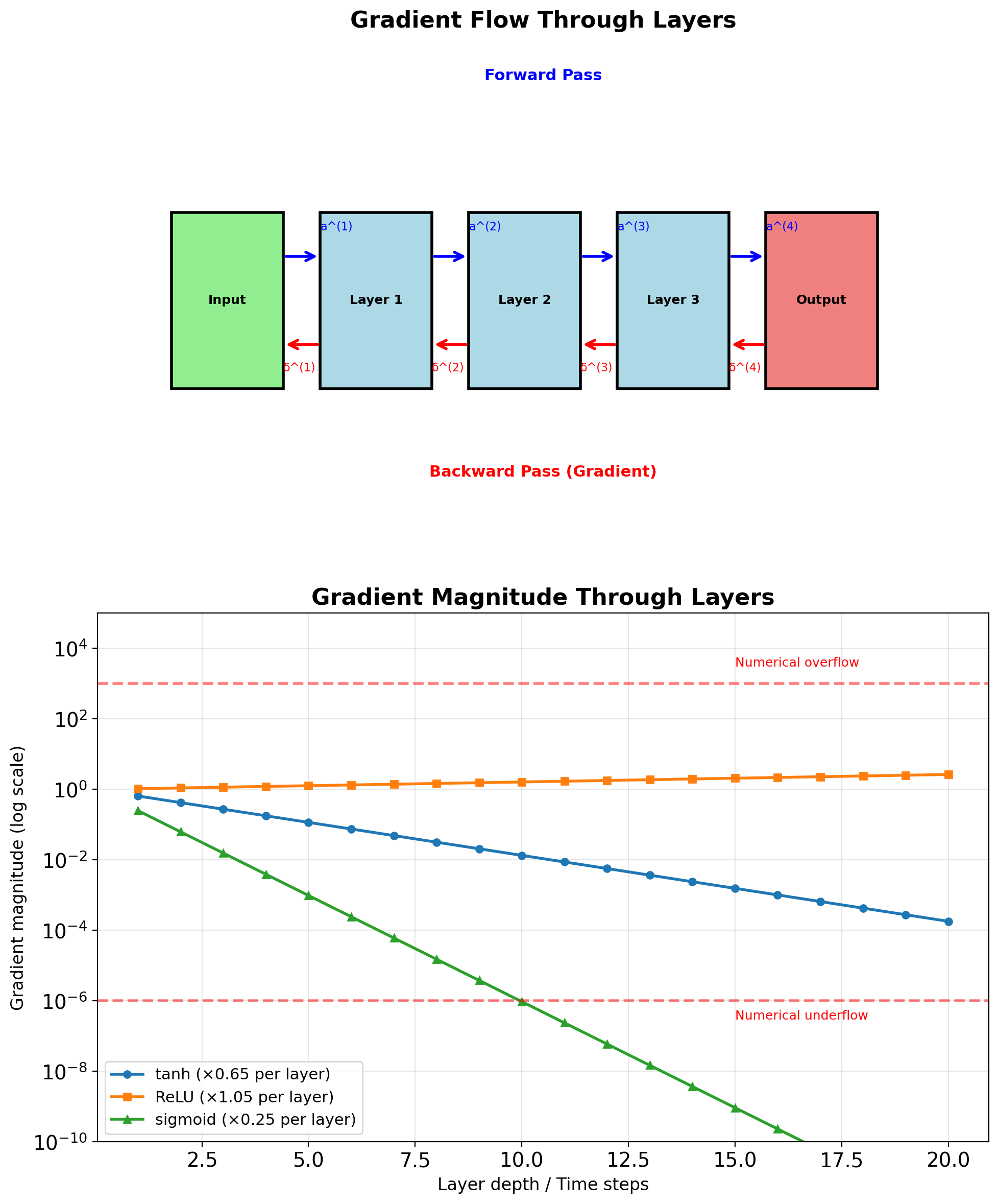
Chain Rule in Deep Networks
For loss \(L\) and parameters \(\mathbf{W}^{(1)}\) in layer 1: \[\frac{\partial L}{\partial \mathbf{W}^{(1)}} = \frac{\partial L}{\partial \mathbf{a}^{(L)}} \cdot \frac{\partial \mathbf{a}^{(L)}}{\partial \mathbf{a}^{(L-1)}} \cdots \frac{\partial \mathbf{a}^{(2)}}{\partial \mathbf{W}^{(1)}}\]
Product of Jacobians: \[\frac{\partial L}{\partial \mathbf{W}^{(1)}} = \boldsymbol{\delta}^{(L)} \prod_{l=2}^{L} \mathbf{J}^{(l)}\]
where \(\mathbf{J}^{(l)} = \frac{\partial \mathbf{a}^{(l)}}{\partial \mathbf{a}^{(l-1)}}\)
Gradient magnitude depends on product of L-1 matrices
For RNNs: Replace depth with time
- \(L\) layers → \(T\) timesteps
- Spatial depth → Temporal depth
Jacobian Matrix Norms
For layer with activation \(\phi\): \[\mathbf{a}^{(l)} = \phi(\mathbf{W}^{(l)}\mathbf{a}^{(l-1)} + \mathbf{b}^{(l)})\]
Jacobian: \[\mathbf{J}^{(l)} = \frac{\partial \mathbf{a}^{(l)}}{\partial \mathbf{a}^{(l-1)}} = \text{diag}(\phi'(\mathbf{z}^{(l)})) \cdot \mathbf{W}^{(l)}\]
Norm bounds: \[\|\mathbf{J}^{(l)}\| \leq \|\phi'\|_{\infty} \cdot \|\mathbf{W}^{(l)}\|\]
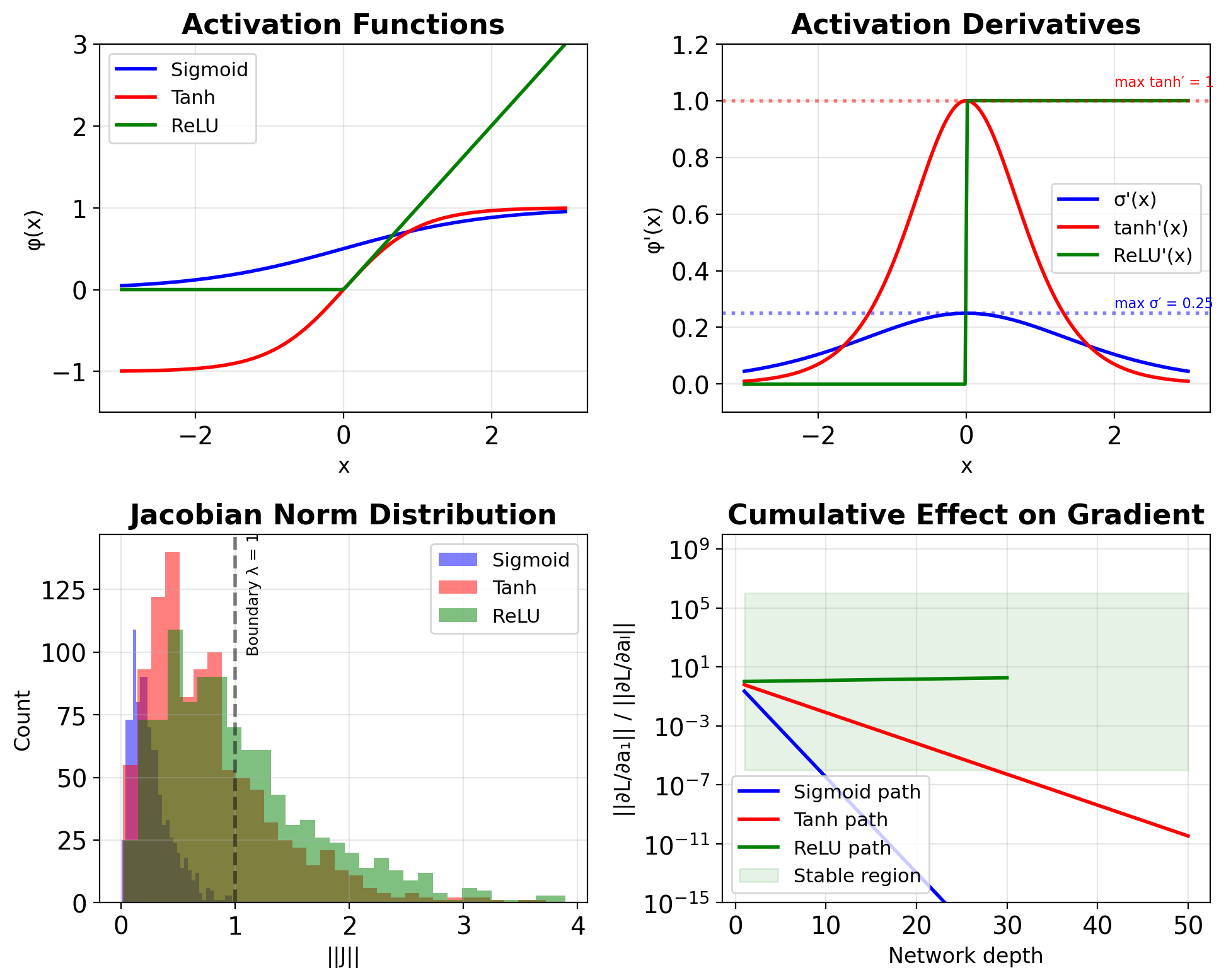
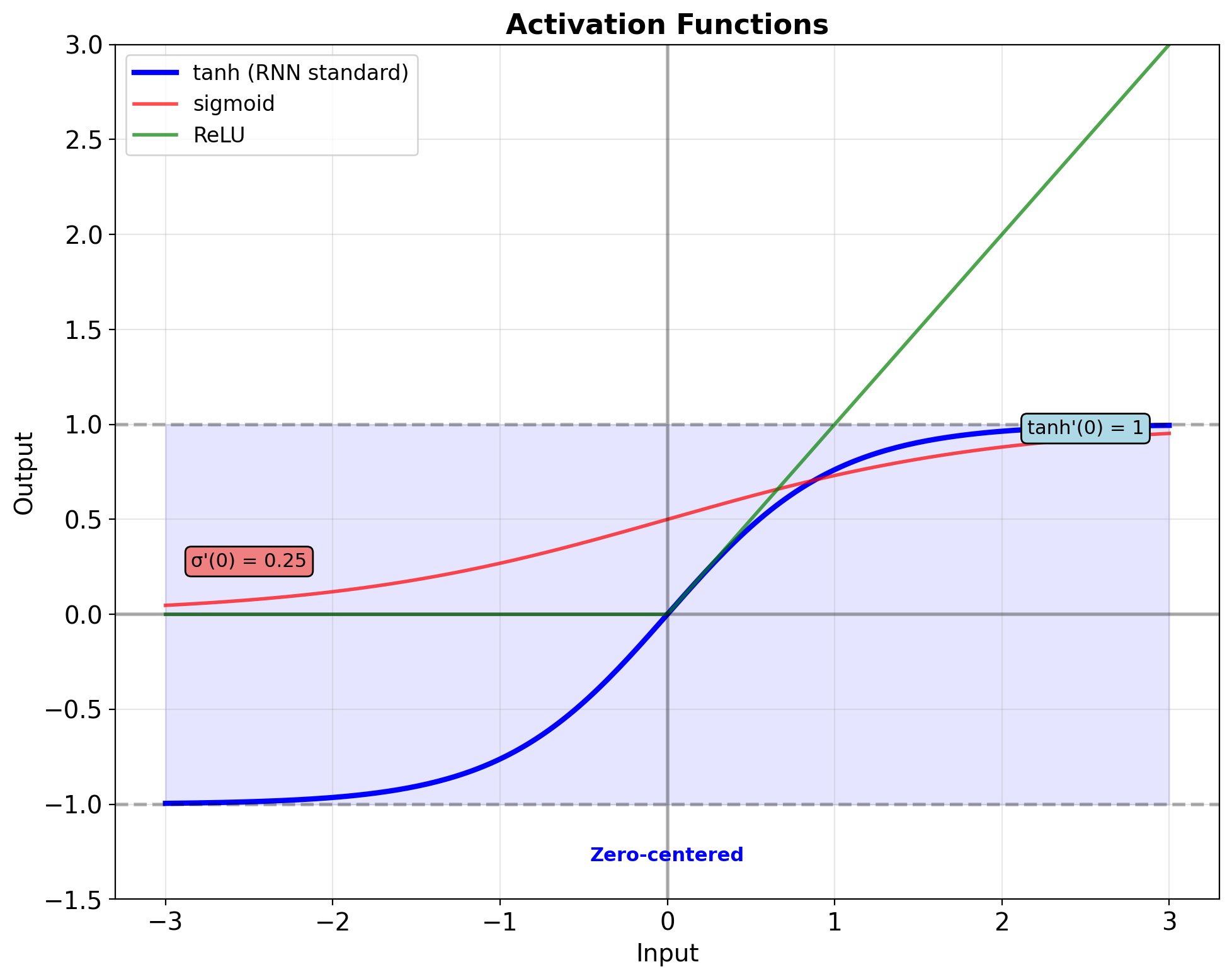
Activation derivatives:
- Sigmoid: \(\sigma'(x) \leq 0.25\)
- Tanh: \(\tanh'(x) \leq 1\)
- ReLU: \(\text{ReLU}'(x) \in \{0, 1\}\)
- Leaky ReLU: \(\text{LReLU}'(x) \in \{\alpha, 1\}\)
Gradient Magnitude Evolution
Starting from loss gradient \(\nabla_{\mathbf{a}^{(L)}} L\): \[\|\nabla_{\mathbf{W}^{(1)}} L\| \approx \|\nabla_{\mathbf{a}^{(L)}} L\| \cdot \prod_{l=2}^{L} \|\mathbf{J}^{(l)}\|\]
Controlling factors:
- Activation function choice
- Weight initialization scale
- Network depth/sequence length
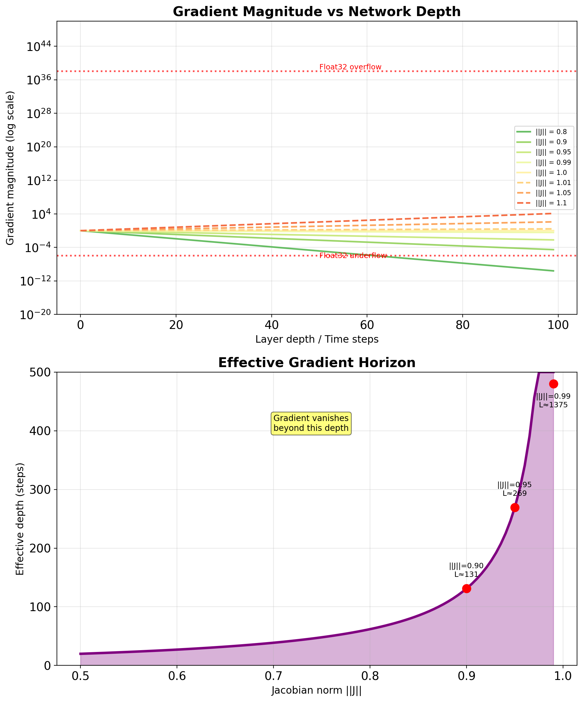
Exponential behavior:
- If \(\prod \|\mathbf{J}\| < 1\): Vanishing (\(e^{-\alpha L}\))
- If \(\prod \|\mathbf{J}\| = 1\): Preserved
- If \(\prod \|\mathbf{J}\| > 1\): Exploding (\(e^{\alpha L}\))
Effective gradient horizon: \[L_{\text{eff}} \approx \frac{\log(\epsilon)}{\log(\|\mathbf{J}\|)}\]
where \(\epsilon\) is numerical precision threshold
The Vanishing Gradient Problem
Sigmoid saturation: \[\sigma'(x) = \sigma(x)(1-\sigma(x)) \leq 0.25\]
Tanh saturation: \[\tanh'(x) = 1 - \tanh^2(x) \leq 1\]
For deep networks:
- 10 layers: \((0.25)^{10} \approx 10^{-6}\)
- 20 layers: \((0.25)^{20} \approx 10^{-12}\)
- 50 layers: \((0.25)^{50} \approx 10^{-30}\)
Consequences:
- Early layers stop learning
- Long-term dependencies lost
- Network depth limited
- Training becomes ineffective
This motivated: ResNets, LSTMs, normalization techniques

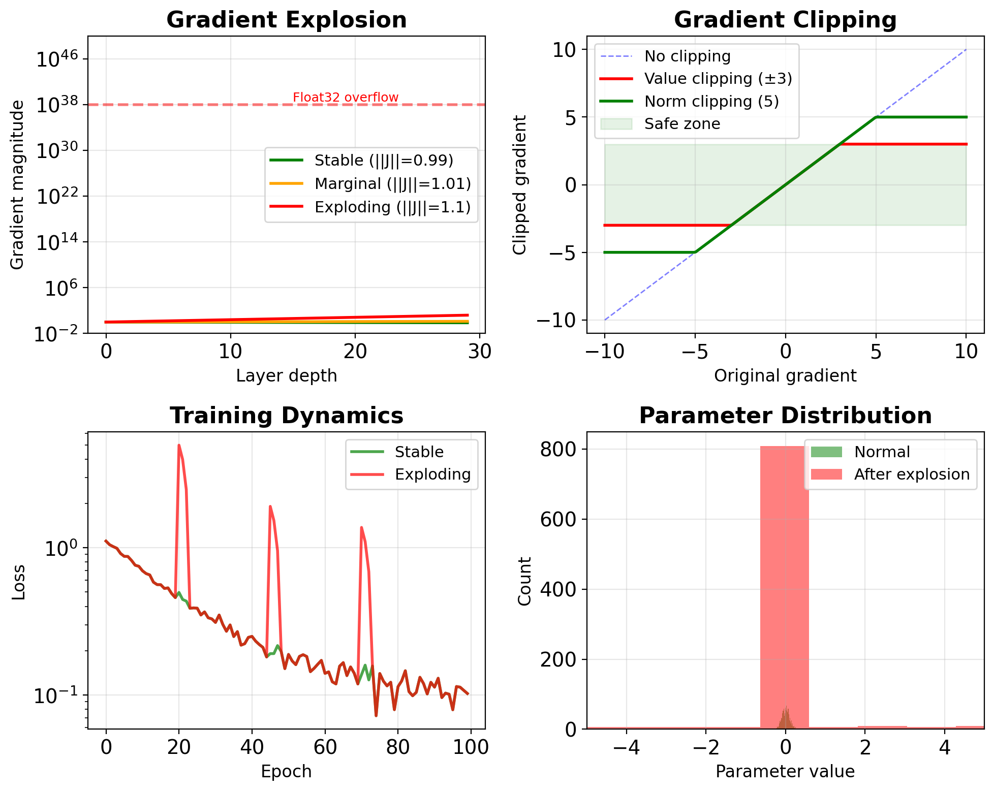
The Exploding Gradient Problem
Causes:
- \(\|\mathbf{W}\| > 1\) with ReLU activation
- Positive feedback loops in RNNs
- Poor initialization
Mathematical analysis: \[\|\nabla\| \approx \|\mathbf{W}\|^L \cdot \|\phi'\|^L\]
For ReLU with \(\|\mathbf{W}\| = 1.5\):
- 10 layers: \((1.5)^{10} \approx 58\)
- 20 layers: \((1.5)^{20} \approx 3,300\)
- 30 layers: \((1.5)^{30} \approx 192,000\)
Consequences:
- Numerical overflow (NaN/Inf)
- Unstable training
- Loss divergence
- Parameter corruption
Solutions: Gradient clipping, careful initialization, normalization
Implications for Temporal Networks
RNN unrolled for T steps = T-layer deep network
Gradient path length: O(T) \[\frac{\partial L}{\partial \mathbf{s}_0} = \prod_{t=1}^T \frac{\partial \mathbf{s}_t}{\partial \mathbf{s}_{t-1}}\]
Challenges scale with sequence length:
- T=10: Manageable
- T=100: Severe vanishing/exploding
- T=1000: Gradient ≈ 0.9^1000 ≈ 10^-46 (underflows)
Effective memory horizon: \[T_{\text{eff}} \approx \frac{1}{1 - \|\mathbf{J}_{\text{RNN}}\|}\]
This motivates:
- Gating mechanisms (LSTM/GRU)
- Attention mechanisms (skip connections in time)
- Truncated BPTT (limit gradient flow)
- Gradient clipping (prevent explosion)
RNN Recurrence Equation
Hidden state update: \[\mathbf{s}_t = \tanh(\mathbf{W}_{ss}\mathbf{s}_{t-1} + \mathbf{W}_{xs}\mathbf{x}_t + \mathbf{b}_s)\]
Output computation: \[\mathbf{y}_t = \mathbf{W}_{sy}\mathbf{s}_t + \mathbf{b}_y\]
- Shared parameters across all timesteps
- Nonlinear state transition via tanh
- Linear output projection
Tanh activation properties:
- Bounded output: [-1, 1] prevents explosion
- Zero-centered: Better gradient flow than sigmoid
- Maximum gradient at origin: tanh’(0) = 1
- Historically standard for RNN stability
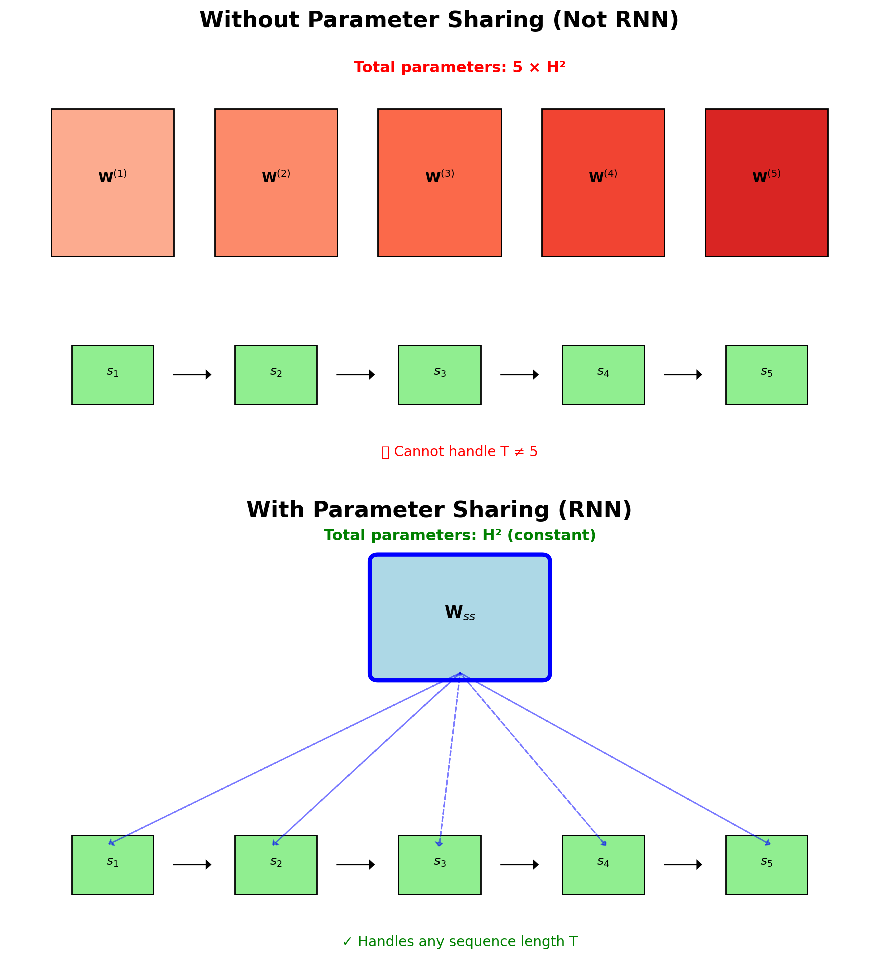
RNNs Share Parameters Across All Timesteps
Without sharing:
- Different weights per timestep: \(\mathbf{W}^{(t)}_{ss}\)
- Parameters grow with sequence: \(O(T \times H^2)\)
- Cannot handle variable length
- No generalization across positions
With sharing (RNN):
- Same weights all timesteps: \(\mathbf{W}_{ss}\)
- Fixed parameters: \(O(H^2)\)
- Handles any sequence length
- Captures position-invariant patterns
CNN shares weights across space; RNN shares across time
- Training: Gradients accumulated across time
- Inference: Can process infinite streams
- Memory: State carries information, not parameters
Unrolled Computation Graph
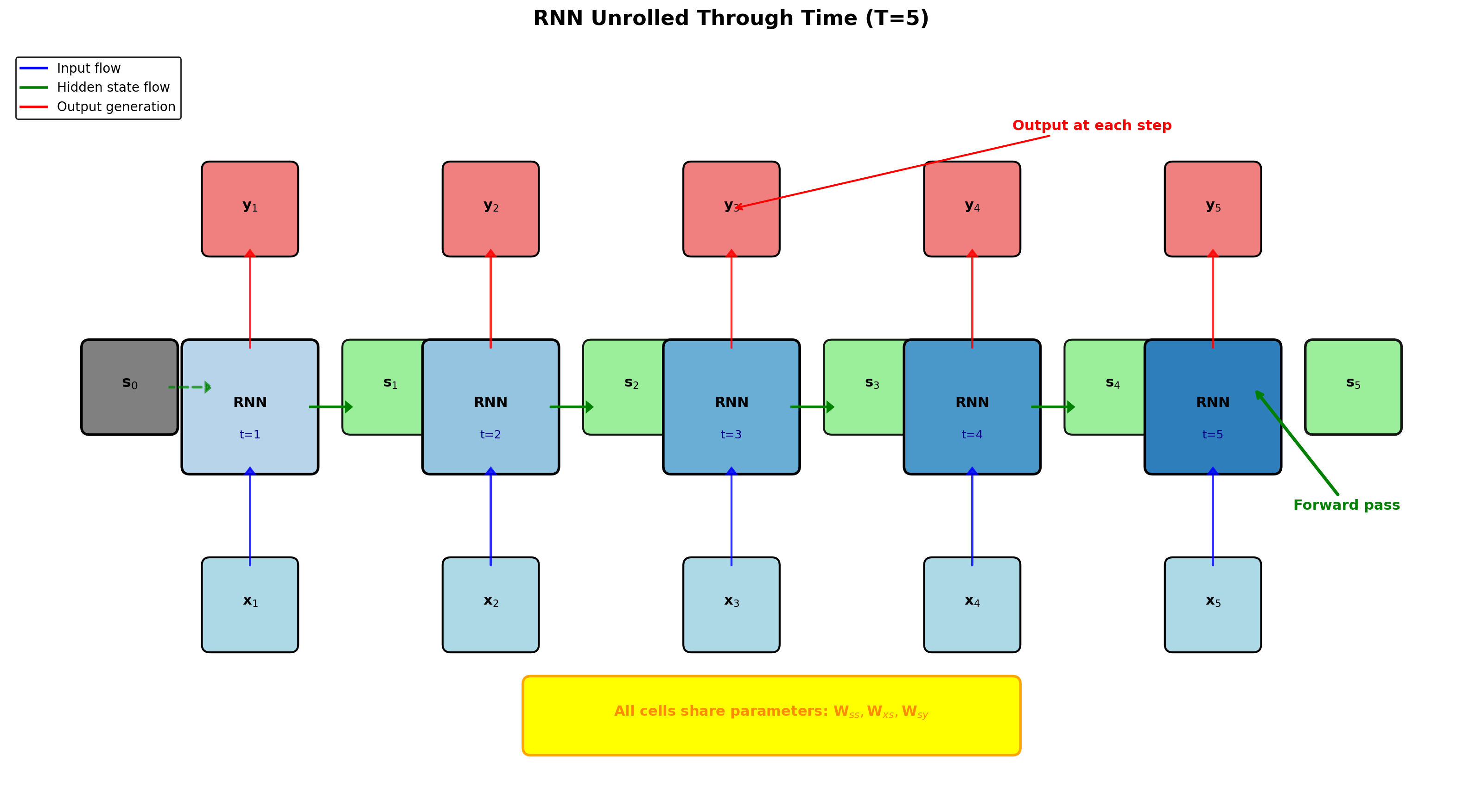
- Each timestep uses same RNN cell (shared parameters)
- Hidden state flows forward carrying temporal information
- Outputs generated independently at each timestep
- Graph depth = sequence length (implications for gradients)
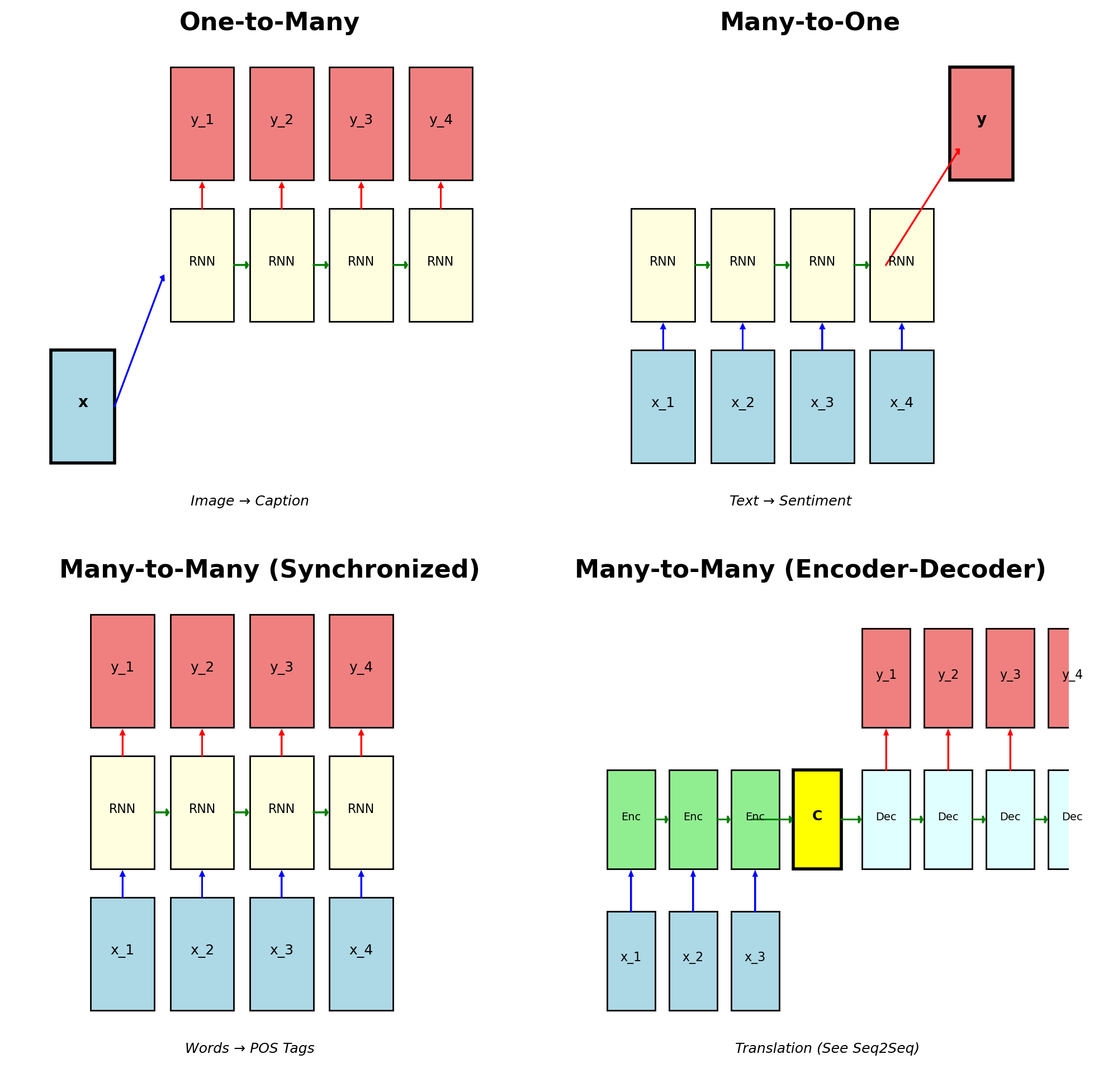
RNNs Support Different Input-Output Configurations
One-to-Many (e.g., image captioning)
- Single input → sequence output
- \(\mathbf{x} \rightarrow \{\mathbf{y}_1, \mathbf{y}_2, ..., \mathbf{y}_T\}\)
Many-to-One (e.g., sentiment analysis)
- Sequence input → single output
- \(\{\mathbf{x}_1, \mathbf{x}_2, ..., \mathbf{x}_T\} \rightarrow \mathbf{y}\)
Many-to-Many (Synchronized) (e.g., POS tagging)
- Aligned input-output sequences
- \(\{\mathbf{x}_t\} \rightarrow \{\mathbf{y}_t\}\), same length
Many-to-Many (Encoder-Decoder) (e.g., translation)
- Different length sequences
- \(\{\mathbf{x}_1, ..., \mathbf{x}_S\} \rightarrow \{\mathbf{y}_1, ..., \mathbf{y}_T\}\)
Encoder-decoder architecture covered in Seq2Seq section
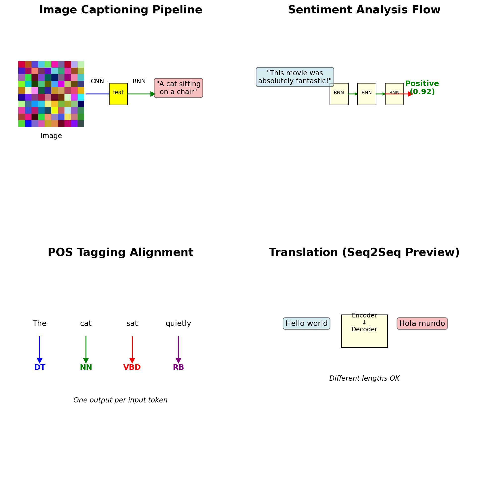
Each RNN Mode Has Specific Real-World Applications
One-to-Many Applications:
- Image captioning: CNN features → word sequence
- Music generation: seed note → melody
- Video description: frame → narrative
Many-to-One Applications:
- Sentiment classification: review → positive/negative
- Spam detection: email → spam/ham
- Activity recognition: sensor sequence → activity
Many-to-Many (Synchronized):
- Part-of-speech tagging: word → POS tag
- Named entity recognition: token → entity type
- Speech recognition: audio frames → phonemes
Many-to-Many (Seq2Seq):
- Machine translation: source → target language
- Summarization: document → summary
- Dialog systems: query → response
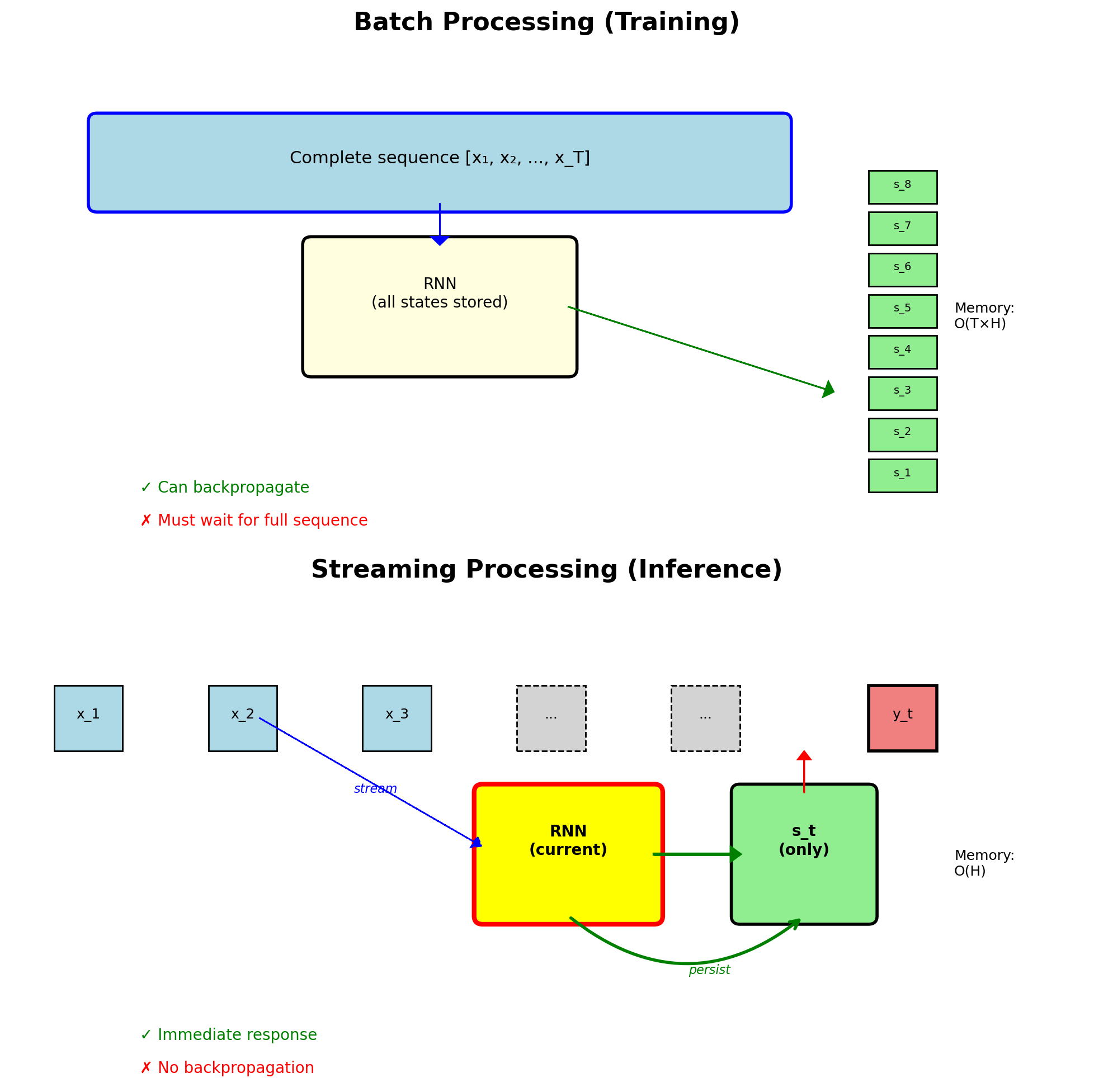
Batch Processing Converts to Streaming Inference
Training mode (fixed length):
- Process complete sequence
- Batch multiple sequences
- Store all hidden states
- Backprop through entire sequence
Streaming mode (infinite length):
- Process one token at a time
- Maintain persistent hidden state
- No storage of history
- Real-time response
Implementation pattern:
# Training (batch)
states = []
for x in sequence:
    h = rnn_cell(h, x)
    states.append(h)

# Streaming (online)
class StreamingRNN:
    def __init__(self):
        self.hidden = None

    def step(self, x):
        if self.hidden is None:
            self.hidden = zeros(H)
        self.hidden = rnn_cell(self.hidden, x)
        return output(self.hidden)
Applications: Live transcription, real-time translation, online monitoring
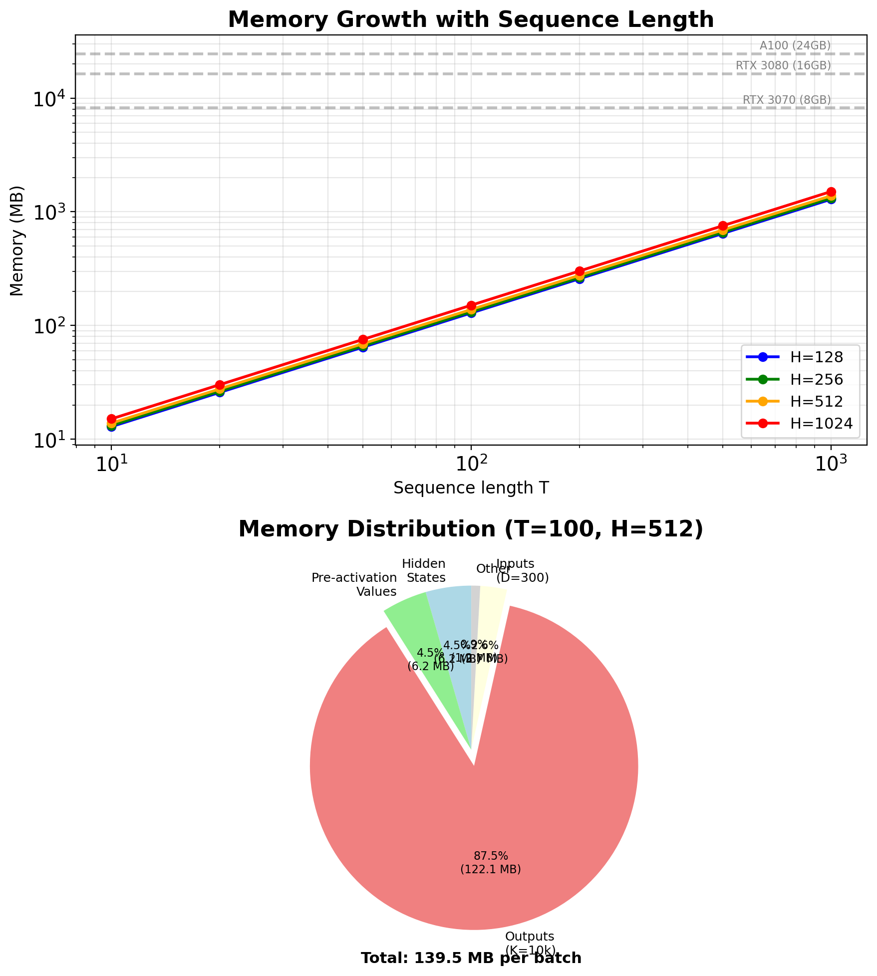
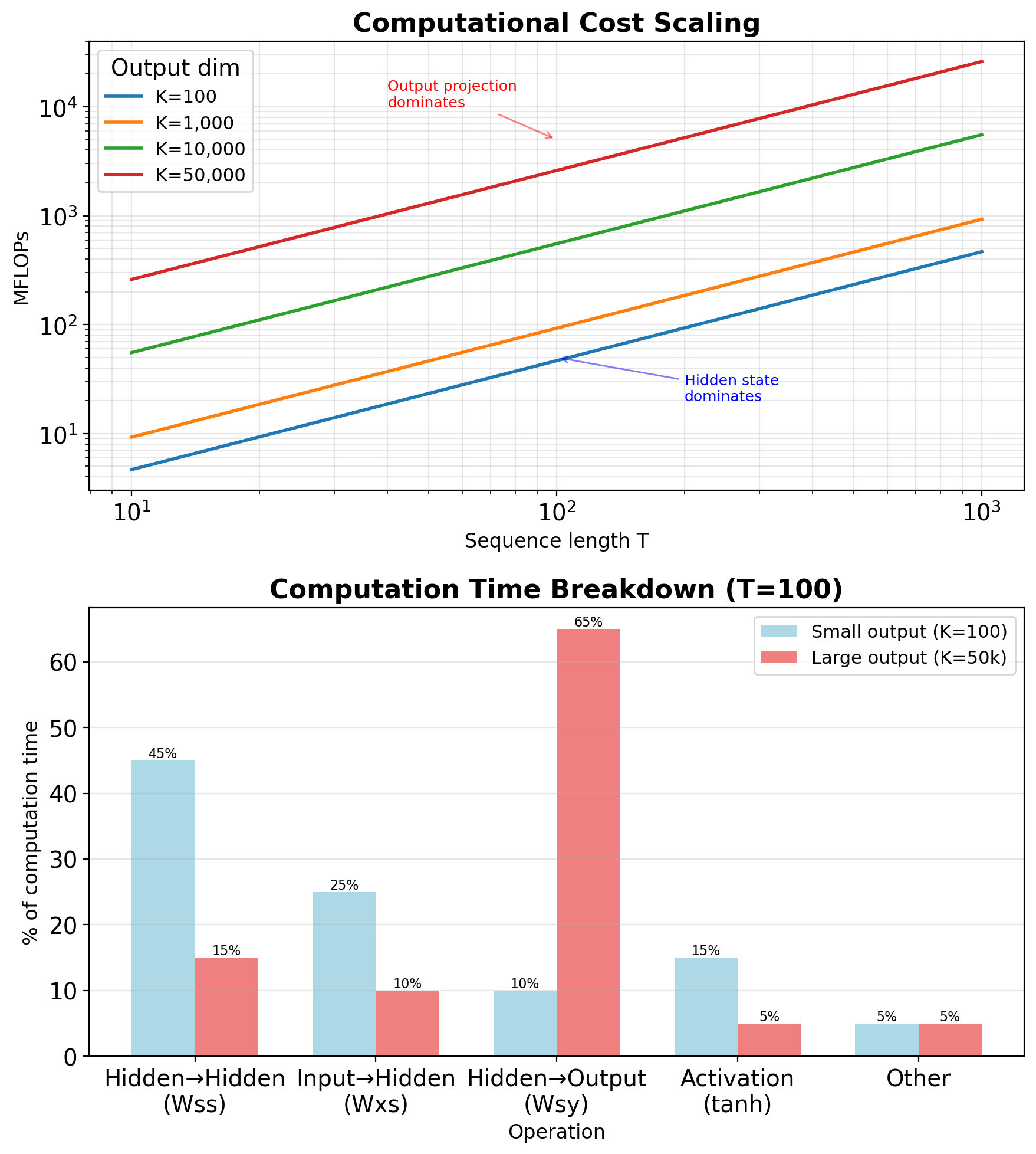
RNN Complexity Scales Linearly with Sequence Length
Matrix multiplications:
- \(\mathbf{W}_{ss} \mathbf{s}_{t-1}\): \(O(H^2)\)
- \(\mathbf{W}_{xs} \mathbf{x}_t\): \(O(HD)\)
- \(\mathbf{W}_{sy} \mathbf{s}_t\): \(O(KH)\)
Per timestep total: \(O(H^2 + HD + KH)\)
Full sequence: \(O(T \times (H^2 + HD + KH))\)
Bottlenecks by task:
- Language modeling (K=50k): Output projection dominates
- Sequence tagging (K=50): Hidden-to-hidden dominates
- Feature extraction (no output): \(H^2\) term dominates
Comparison with Transformers:
- RNN: \(O(T \times H^2)\) sequential
- Transformer: \(O(T^2 \times H)\) parallel
- Crossover point: T ≈ H
Parallelization constraints:
- Each step needs previous state
- No independence across time
- GPU underutilized (low parallelism)

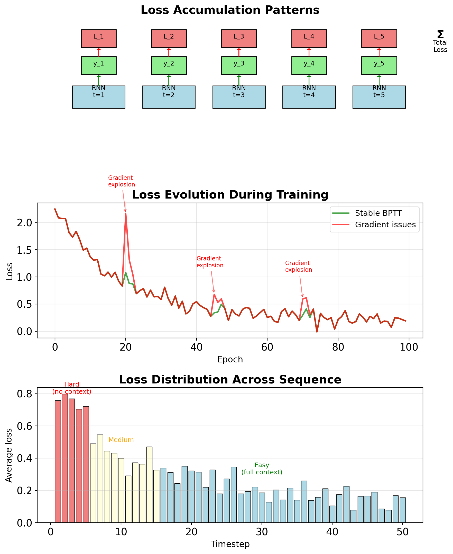
Sequence-Level Loss Computation
Total loss: \[L = \sum_{t=1}^T L_t(\mathbf{y}_t, \hat{\mathbf{y}}_t)\]
Common loss functions:
Classification: Cross-entropy per timestep \[L_t = -\sum_{k=1}^K y_{tk} \log \hat{y}_{tk}\]
Regression: MSE per timestep \[L_t = \|\mathbf{y}_t - \hat{\mathbf{y}}_t\|^2\]
Language modeling: Perplexity \[\text{PPL} = \exp\left(\frac{1}{T}\sum_t L_t\right)\]
Loss accumulation patterns:
- All timesteps (many-to-many): Sum all \(L_t\)
- Final timestep (many-to-one): Only \(L_T\)
- Masked positions: \(\sum_t m_t L_t\) where \(m_t \in \{0,1\}\)
Gradient starts from: \[\frac{\partial L}{\partial \mathbf{y}_t} = \frac{\partial L_t}{\partial \mathbf{y}_t}\]
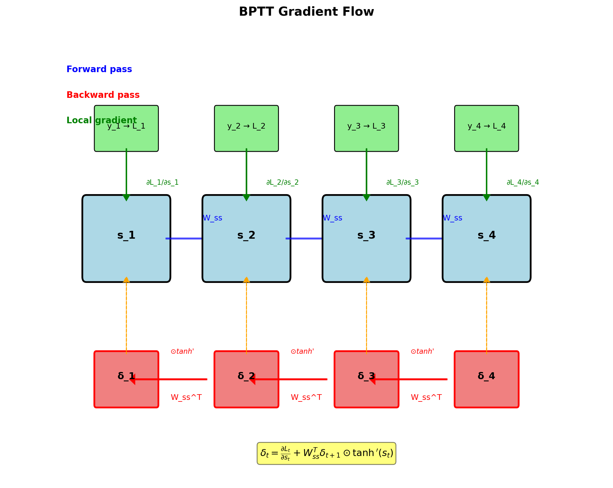
BPTT Gradient Recursion
Error signal at hidden state: \[\boldsymbol{\delta}_t = \frac{\partial L}{\partial \mathbf{s}_t}\]
Recursive computation: \[\boldsymbol{\delta}_t = \frac{\partial L_t}{\partial \mathbf{s}_t} + \mathbf{W}_{ss}^T \boldsymbol{\delta}_{t+1} \odot \tanh'(\mathbf{s}_t)\]
Components:
- Local gradient: \(\frac{\partial L_t}{\partial \mathbf{s}_t} = \mathbf{W}_{sy}^T \frac{\partial L_t}{\partial \mathbf{y}_t}\)
- Future gradient: \(\mathbf{W}_{ss}^T \boldsymbol{\delta}_{t+1}\)
- Activation derivative: \(\tanh'(\mathbf{s}_t) = 1 - \tanh^2(\mathbf{s}_t)\)
Boundary condition: \[\boldsymbol{\delta}_T = \frac{\partial L_T}{\partial \mathbf{s}_T}\]
Gradient flows backward through same path as forward state flow
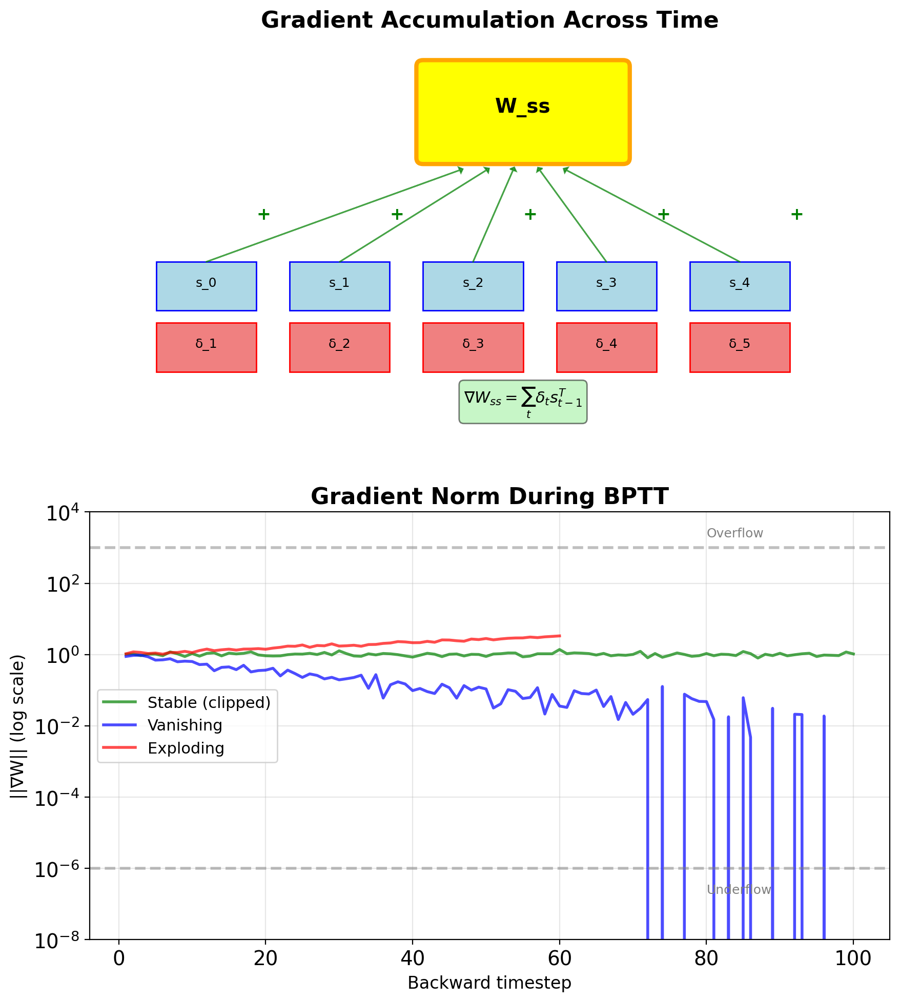
Gradient w.r.t. Weights
Weight gradient accumulation
Hidden-to-hidden weights: \[\frac{\partial L}{\partial \mathbf{W}_{ss}} = \sum_{t=1}^T \boldsymbol{\delta}_t \mathbf{s}_{t-1}^T\]
Input-to-hidden weights: \[\frac{\partial L}{\partial \mathbf{W}_{xs}} = \sum_{t=1}^T \boldsymbol{\delta}_t \mathbf{x}_t^T\]
Hidden-to-output weights: \[\frac{\partial L}{\partial \mathbf{W}_{sy}} = \sum_{t=1}^T \frac{\partial L_t}{\partial \mathbf{y}_t} \mathbf{s}_t^T\]
- Gradients sum across all timesteps
- Same weights receive gradients from entire sequence
- Long sequences → many gradient contributions
- Can lead to gradient explosion if not controlled
Computational pattern:
Computational Graph for BPTT

Truncated BPTT
Limiting gradient flow for efficiency
Motivation:
- Full BPTT: O(T²) memory and time
- Gradient vanishing makes long BPTT ineffective
- Need to process very long sequences
Truncated BPTT algorithm:
- Forward pass: Process full sequence
- Backward pass: Only last k steps
- Detach gradient at truncation point
def truncated_bptt(sequence, k=20):
    states = []
    for t in range(len(sequence)):
        if t % k == 0:
            # Detach: stop gradient flow
            state = state.detach()
        state = rnn_cell(state, sequence[t])
        states.append(state)

        if t % k == k-1:
            # Backprop through last k steps
            loss = compute_loss(states[-k:])
            loss.backward()
Trade-offs:
- k small (5-10): Fast but poor long-range
- k medium (20-35): Good balance
- k large (50+): Slow, diminishing returns

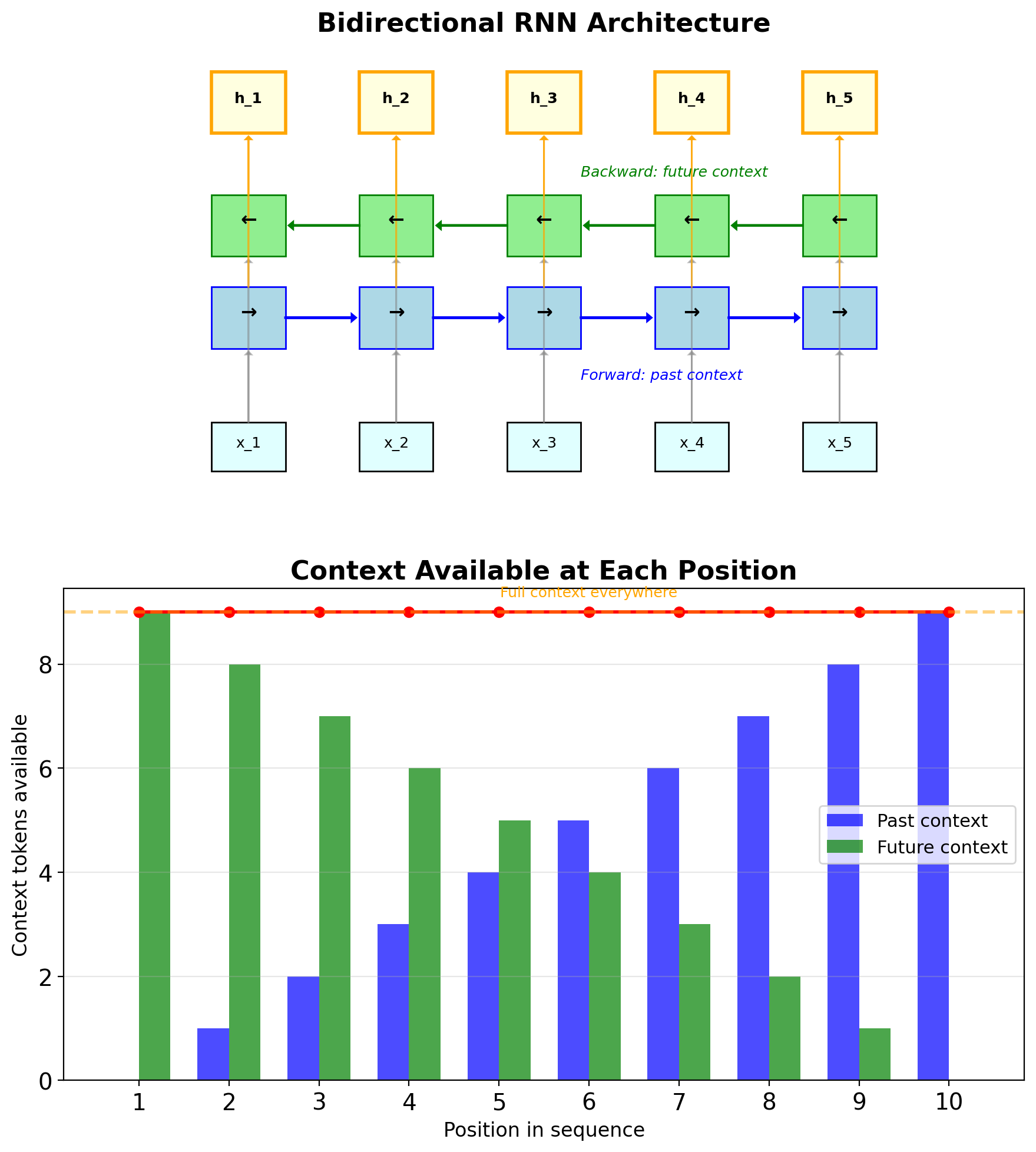
Bidirectional RNNs
Processing sequences in both directions
Architecture:
- Forward RNN: Processes \(x_1, x_2, ..., x_T\)
- Backward RNN: Processes \(x_T, x_{T-1}, ..., x_1\)
- Concatenate or sum hidden states
\[\vec{\mathbf{s}}_t = \text{RNN}_{\rightarrow}(x_t, \vec{\mathbf{s}}_{t-1})\] \[\overleftarrow{\mathbf{s}}_t = \text{RNN}_{\leftarrow}(x_t, \overleftarrow{\mathbf{s}}_{t+1})\] \[\mathbf{s}_t = [\vec{\mathbf{s}}_t; \overleftarrow{\mathbf{s}}_t]\]
- Full context at every position
- Better for sequence labeling
- 2× parameters and computation
Limitations:
- Cannot use for online/streaming
- Need full sequence before processing
- Not suitable for generation tasks
# PyTorch implementation
birnn = nn.RNN(input_size, hidden_size,
              bidirectional=True,
              batch_first=True)
# Output size: (batch, seq_len, 2*hidden_size)
Common applications:
- Named entity recognition
- Part-of-speech tagging
- Speech recognition (offline)
Formal Bound on Gradient Norm
Starting from: \[\left\|\frac{\partial \mathbf{s}_t}{\partial \mathbf{s}_{t-1}}\right\| = \|\text{diag}(\tanh'(\mathbf{z}_t)) \cdot \mathbf{W}_{ss}\|\]
Using submultiplicativity: \[\left\|\frac{\partial \mathbf{s}_t}{\partial \mathbf{s}_{t-1}}\right\| \leq \|\text{diag}(\tanh'(\mathbf{z}_t))\| \cdot \|\mathbf{W}_{ss}\|\]
Bounds:
- \(\|\text{diag}(\tanh'(\mathbf{z}_t))\| = \max_i |\tanh'(z_i)| \leq 1\)
- Define \(\gamma = \|\mathbf{W}_{ss}\| \cdot \max_t \|\text{diag}(\tanh'(\mathbf{z}_t))\|\)
Final bound: \[\left\|\frac{\partial L}{\partial \mathbf{s}_k}\right\| \leq \gamma^{T-k} \left\|\frac{\partial L}{\partial \mathbf{s}_T}\right\|\]
Gradient behavior depends on \(\gamma^{T-k}\):
- \(\gamma < 1\): Gradients decay as \(\gamma^{T-k} \rightarrow 0\)
- \(\gamma > 1\): Gradients grow as \(\gamma^{T-k} \rightarrow \infty\)
- Effective memory: \(T_{eff} \approx \log(\epsilon)/\log(\gamma)\) steps
Empirically measured:
- Vanilla RNN: 10-20 steps effective memory
- Copy task: Performance drops to chance after ~15 steps
- Language modeling: Effective range 10-20 words (Bengio et al., 1994)

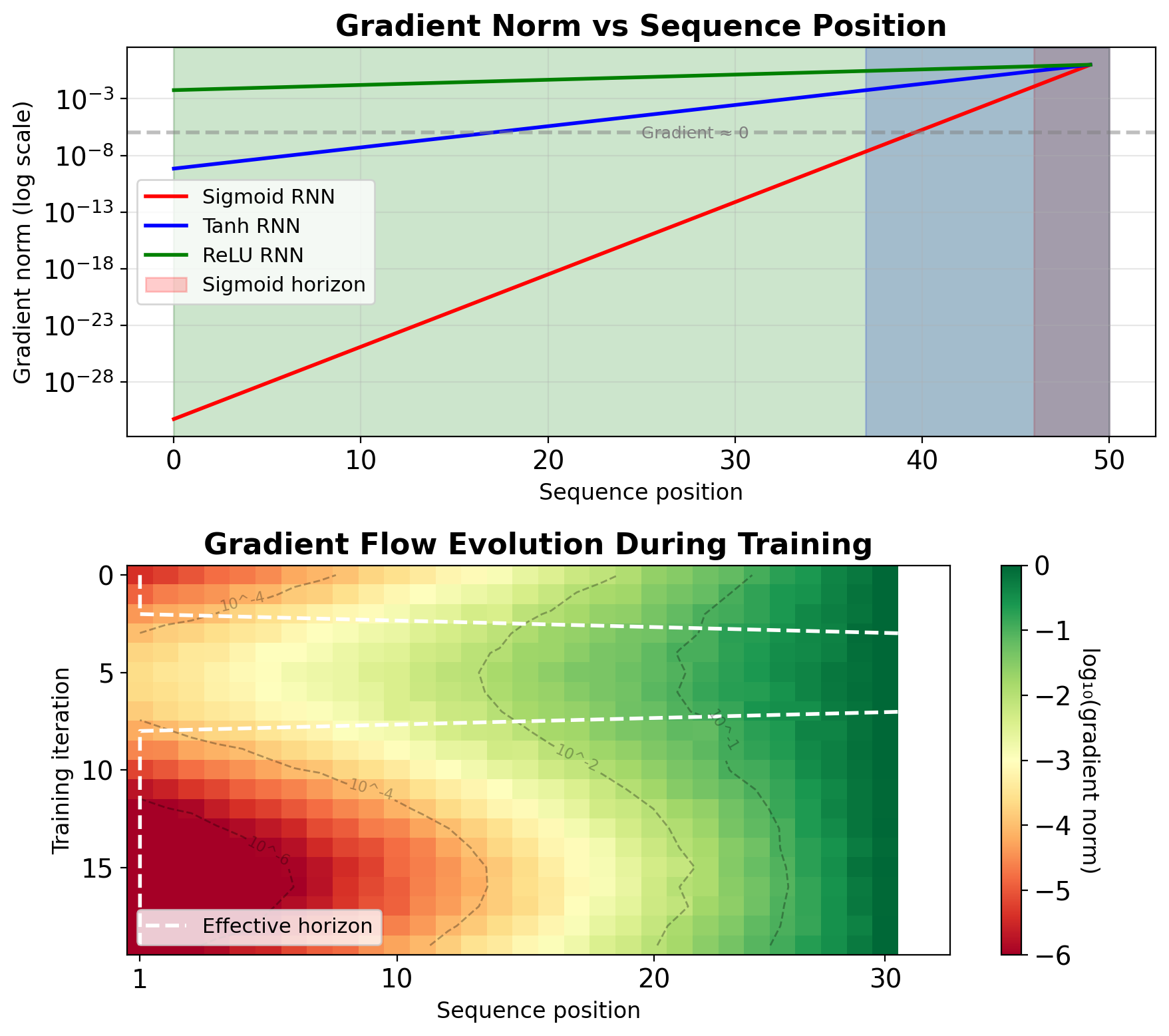
Gradients Decay Exponentially with Time Steps
Experiment setup:
- Train RNN on sequence length T=100
- Measure gradient norm at each position
- Track over training iterations
- Distance effect: \(\|\nabla_{\mathbf{s}_k}\| \propto \gamma^{T-k}\)
- Effective horizon: ~10-20 steps for vanilla RNN
- Network ignores early inputs
Measured decay rates:
- Sigmoid RNN: \(\gamma \approx 0.23\) → T_eff ≈ 4 steps
- Tanh RNN: \(\gamma \approx 0.65\) → T_eff ≈ 13 steps
- ReLU RNN: \(\gamma \approx 0.9\) → T_eff ≈ 63 steps (but unstable)
Practical implication: Cannot learn dependencies beyond T_eff
Training Dynamics Show Rapid Gradient Attenuation
Setup: Penn Treebank language modeling
# Model configuration
hidden_size = 128
num_layers = 1
sequence_length = 35
vocab_size = 10000

# Training
batch_size = 32
learning_rate = 1.0
Gradient measurements:
- Average over 100 batches
- Track position-wise gradient norms
- Compare different architectures
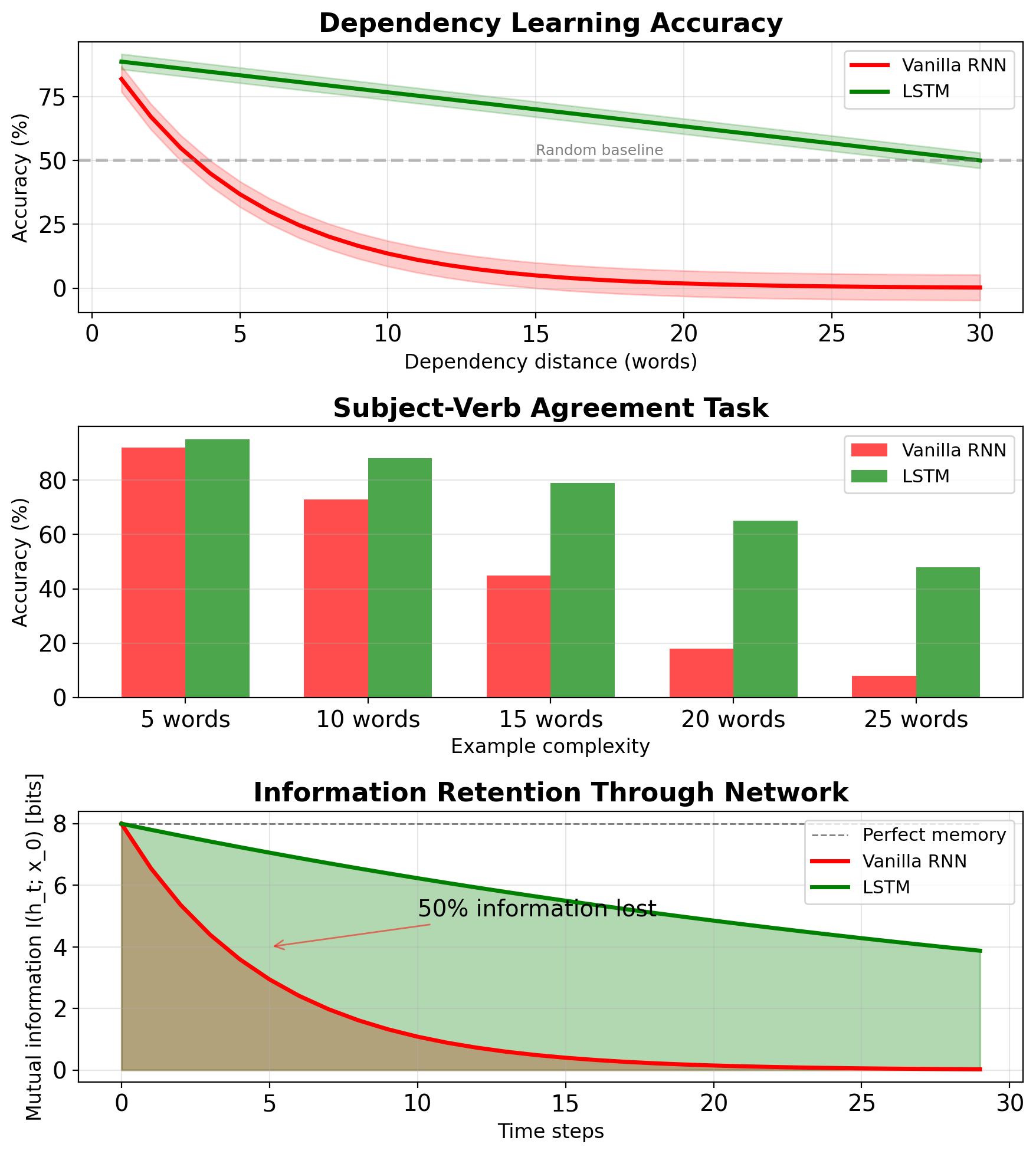
Results:
- Vanilla RNN: 90% gradient loss after 15 steps
- Layer norm helps: Extends to ~25 steps
- Still inadequate: Language needs 50+ steps
- LSTM necessary: Maintains gradients 100+ steps
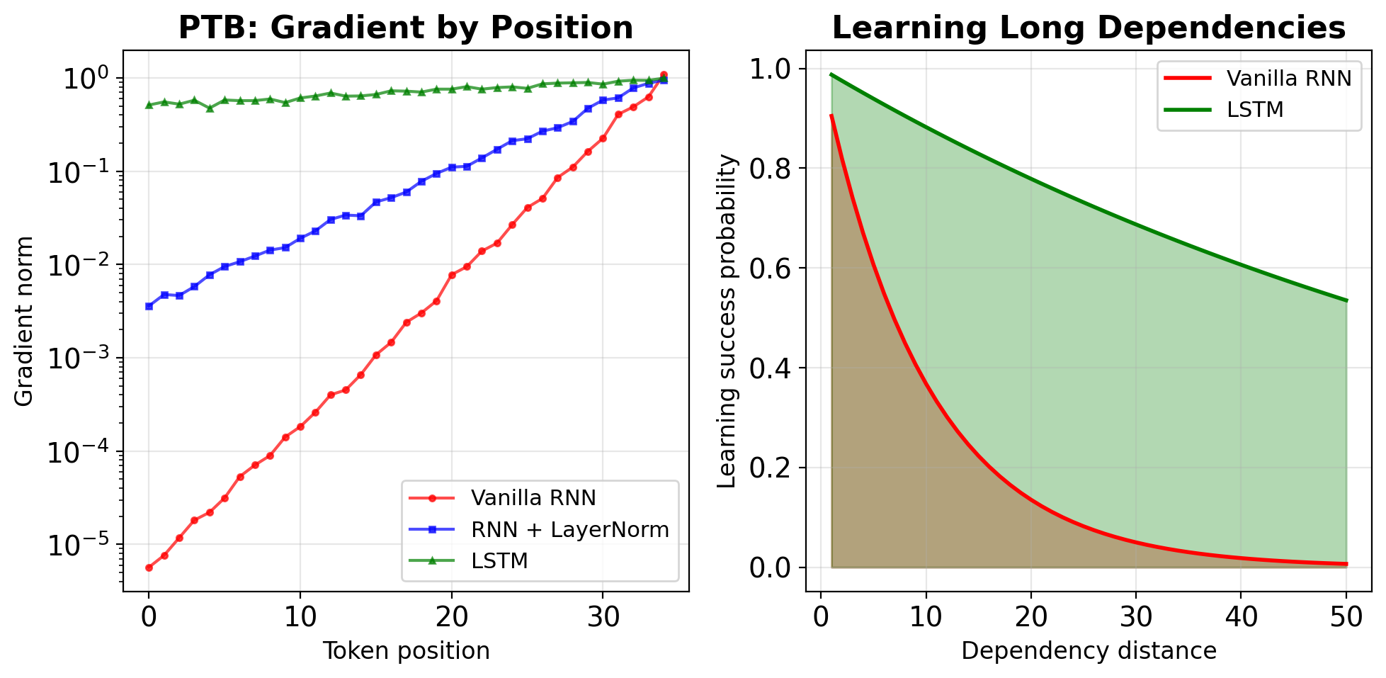
Vanishing Gradients Limit Long-Term Dependencies
Observable behaviors:
- Recency bias: Recent inputs dominate
- Ignored prefixes: Early tokens have no impact
- Short-range patterns only: N-grams, not syntax
Quantified impact (word prediction task):
Dependency | Vanilla RNN | LSTM
-----------|-------------|------
1-5 words  | 85% acc    | 87% acc
5-10 words | 45% acc    | 78% acc
10-20 words| 12% acc    | 65% acc
20+ words  | ~random    | 43% acc
Failure modes:
- Cannot track subject-verb agreement > 15 words
- Forgets context in long sentences
- Cannot maintain coherent topic
Compensation strategies (inadequate):
- Increase hidden size → Memory cost
- Reduce sequence length → Lose context
- Curriculum learning → Limited improvement
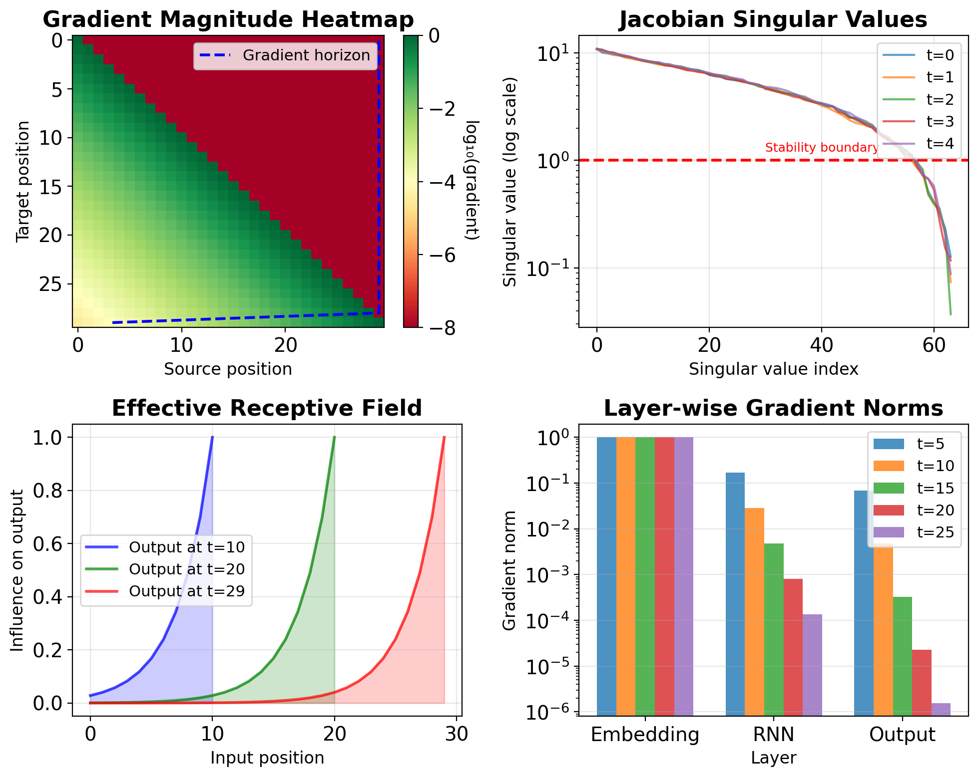
Gradient Flow Visualization Reveals Bottlenecks
Techniques for visualization:
- Gradient magnitude heatmaps
- Jacobian singular values
- Effective receptive field
- Layer-wise gradient norms
Gradient behavior:
- Gradient cliff: Sharp drop after 10-15 steps
- Dead zones: Positions with ||∇|| < 1e-6
- Asymmetric flow: Later positions dominate
Diagnostic metrics: \[\text{Gradient ratio} = \frac{\|\nabla_{\mathbf{s}_0}\|}{\|\nabla_{\mathbf{s}_T}\|}\]
Typical values:
- Vanilla RNN: 10^(-6) to 10^(-10)
- With gradient clipping: 10^(-4) to 10^(-6)
- LSTM: 10^(-1) to 10^(-3)
Interpretation: Information cannot flow backward beyond the gradient horizon
Gradients Explode When Spectral Radius Exceeds Unity
\[\left\|\frac{\partial \mathbf{s}_t}{\partial \mathbf{s}_{t-1}}\right\| = \|\text{diag}(f'(\mathbf{z}_t)) \cdot \mathbf{W}_{ss}\| > 1\]
When this happens:
- Large weight initialization: \(\|\mathbf{W}_{ss}\| > 1\)
- ReLU with positive feedback: No saturation to limit growth
- Adversarial parameter combinations: Gradients explode despite proper initialization
Explosion characteristics:
- Sudden onset (fine → explosion in 1 step)
- Numerical overflow: NaN/Inf values
- Loss spikes to infinity
- Training completely fails
Measured explosion rates:
- \(\|\mathbf{J}\| = 1.1\): Explodes after ~70 steps
- \(\|\mathbf{J}\| = 1.5\): Explodes after ~15 steps
- \(\|\mathbf{J}\| = 2.0\): Explodes after ~8 steps

Two Standard Methods for Gradient Clipping
1. Value clipping (element-wise):
2. Norm clipping (preserve direction):
def clip_grad_norm(grads, max_norm):
    total_norm = torch.sqrt(
        sum(g.norm()**2 for g in grads))
    clip_coef = max_norm / (total_norm + 1e-6)
    clip_coef = min(clip_coef, 1.0)
    for g in grads:
        g.mul_(clip_coef)
    return total_norm
Comparison:
- Value: Simple, can distort direction
- Norm: Preserves direction, standard for RNNs
- Adaptive: Threshold adjusts during training
Norm Clipping Rescales Gradient Direction
Basic norm clipping:
Complete training loop:
def train_step(model, data, target, clip_val=5.0):
    optimizer.zero_grad()
    output = model(data)
    loss = criterion(output, target)
    loss.backward()

    # Clip gradients
    total_norm = torch.nn.utils.clip_grad_norm_(
        model.parameters(), clip_val)

    # Monitor gradient explosion
    if total_norm > clip_val:
        print(f"Clipped: {total_norm:.2f} -> {clip_val}")

    optimizer.step()
    return loss.item(), total_norm.item()
Adaptive clipping:
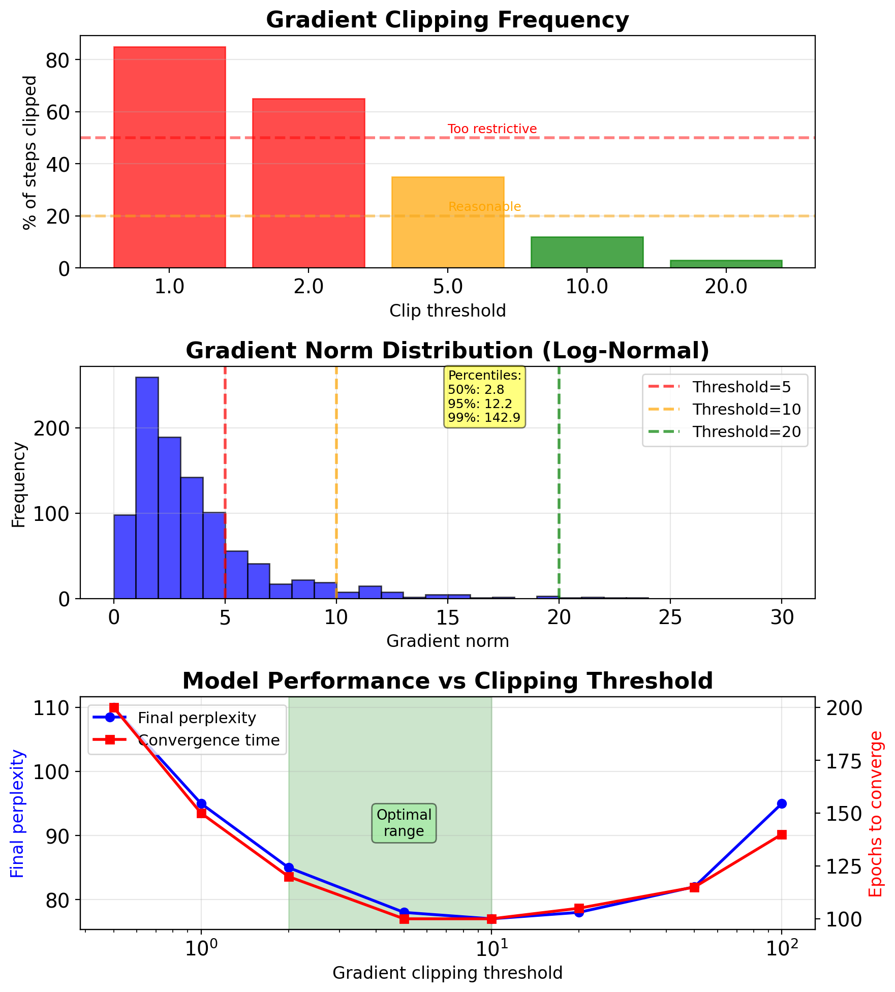
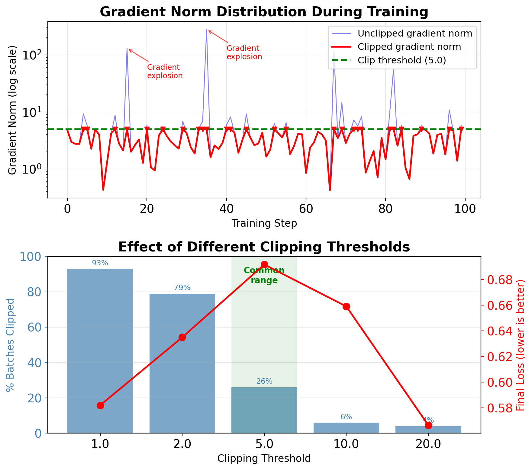
Clipping Threshold Requires Empirical Tuning
Empirical guidelines:
- Start with 5.0-10.0 for most tasks
- Language models: 1.0-5.0
- Sequence-to-sequence: 5.0-10.0
- RL tasks: 0.5-1.0 (more sensitive)
Monitoring strategy:
# Track clipping statistics
clip_stats = {
    'total_steps': 0,
    'clipped_steps': 0,
    'max_norm_seen': 0,
    'avg_norm': 0
}

# Log percentage clipped
if total_norm > max_norm:
    clip_stats['clipped_steps'] += 1
Warning signs:
50% steps clipped → threshold too low
- <1% steps clipped → threshold too high
- Sudden spike in clipping → check learning rate
Adaptive strategies:
- Percentile-based: Set to 95th percentile
- Moving average: 3× running average
- Schedule: Decrease over training
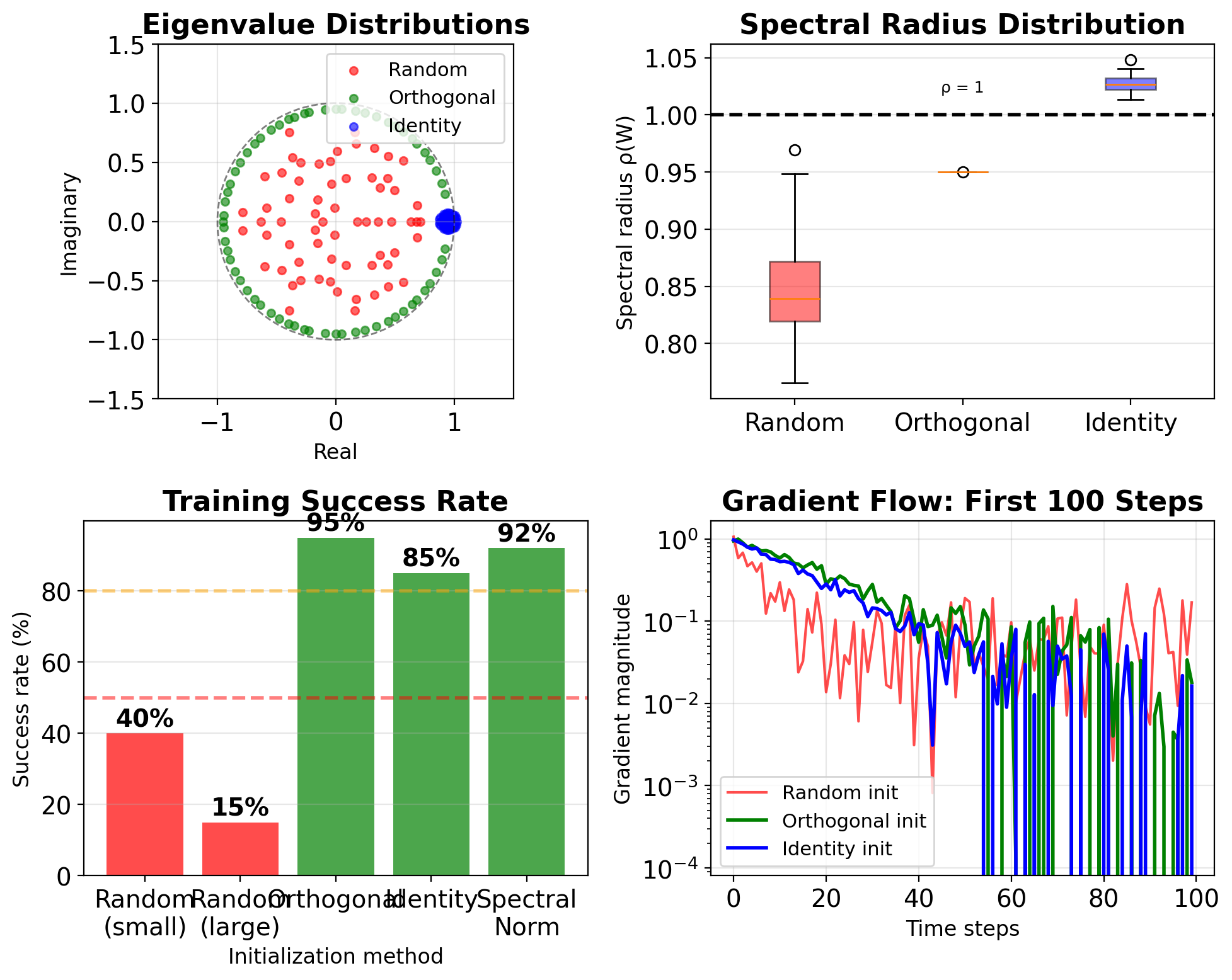
RNN Initialization Prevents Early Divergence
1. Orthogonal initialization:
def orthogonal_init(weight):
    nn.init.orthogonal_(weight)
    # Ensure spectral radius < 1
    with torch.no_grad():
        weight *= 0.95
2. Identity initialization (IRNN):
3. Spectral normalization:
def spectral_normalize(weight, target=0.95):
    with torch.no_grad():
        s = torch.svd(weight).S[0]
weight *= target / s- Orthogonal: Preserves gradient norm initially
- Identity: Simple dynamics, easier debugging
- Spectral: Direct control of largest eigenvalue
Empirical results (Penn Treebank):
- Random init: 60% training failures
- Orthogonal: 5% failures
- Identity: 10% failures
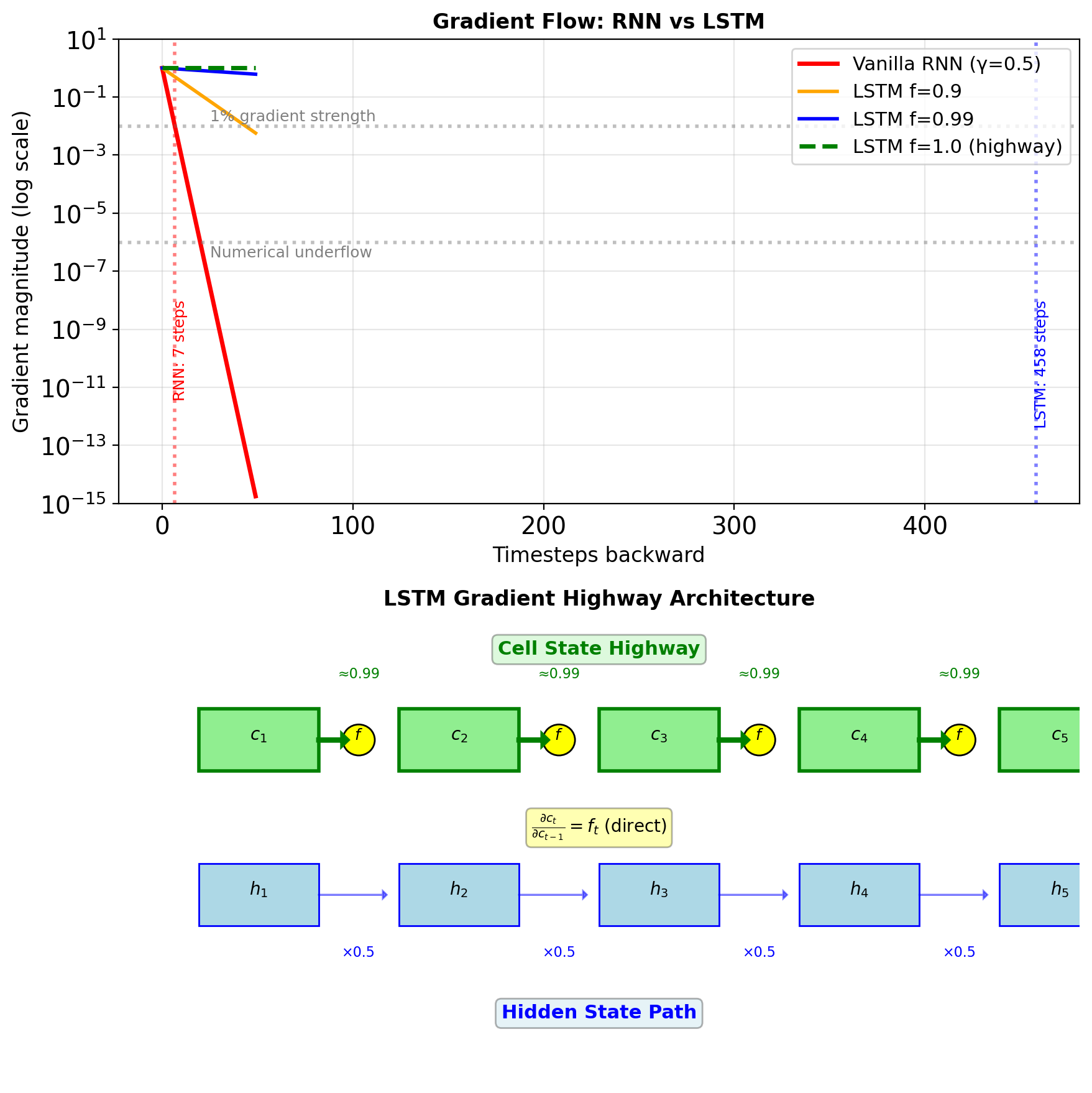
Gates Create Gradient Highways Through Time
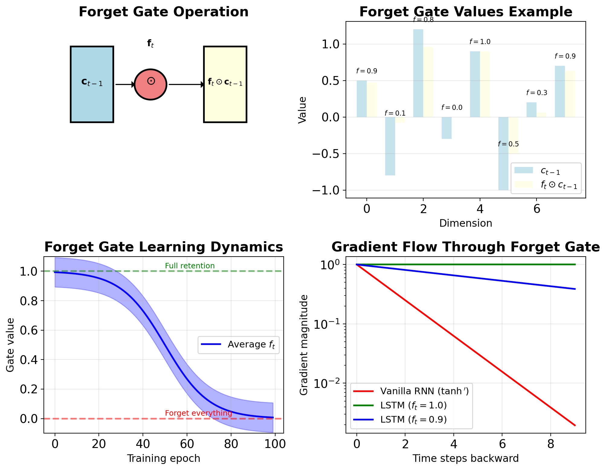
\[\frac{\partial L}{\partial \mathbf{s}_0} = \prod_{t=1}^T \underbrace{\|\mathbf{W}\| \cdot |\tanh'|}_{\leq 0.5} \approx 0.5^T\]
After 20 steps: \(0.5^{20} \approx 10^{-6}\) (vanished!)
LSTM’s solution: Create bypass paths
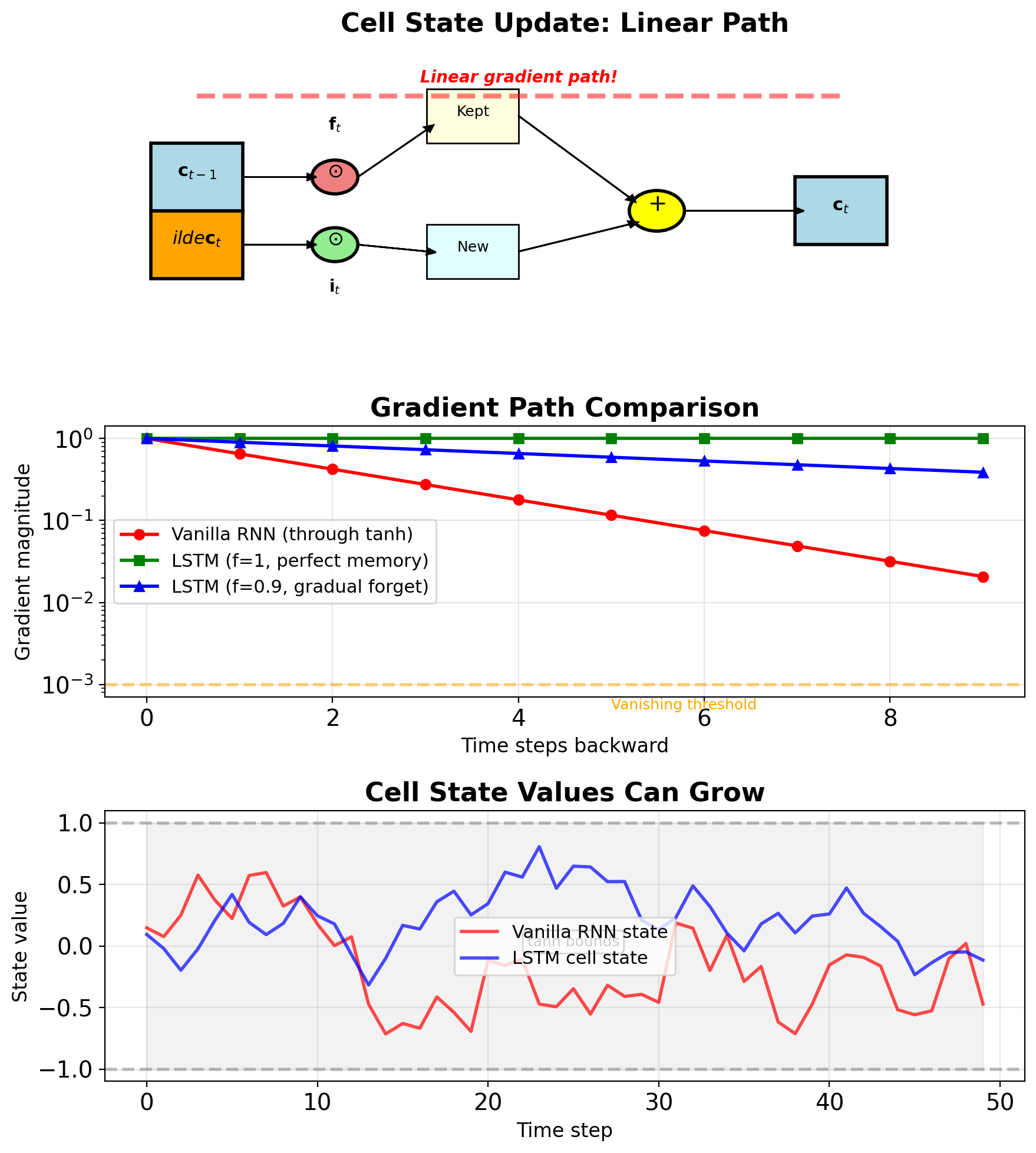
Cell state gradient: \[\frac{\partial \mathbf{c}_t}{\partial \mathbf{c}_{t-1}} = \mathbf{f}_t + \text{other terms}\]
When \(\mathbf{f}_t \approx 1\): Linear path through time!
Gates control gradient flow:
- \(\mathbf{f}_t = 0.9\): Gradient decays as \(0.9^T\)
- \(\mathbf{f}_t = 0.99\): Gradient decays as \(0.99^T\)
- \(\mathbf{f}_t = 1.0\): No decay (highway)
Practical impact:
- Vanilla RNN: 10-20 step memory
- LSTM: 100+ step memory
- Difference: \(0.5^{100}\) vs \(0.99^{100}\) = \(10^{-30}\) vs \(0.37\)
LSTM Gates Preserve Gradient Magnitude
\[\frac{\partial L}{\partial \mathbf{c}_{t-1}} = \frac{\partial L}{\partial \mathbf{c}_t} \cdot \frac{\partial \mathbf{c}_t}{\partial \mathbf{c}_{t-1}}\]
Cell state update equation: \[\mathbf{c}_t = \mathbf{f}_t \odot \mathbf{c}_{t-1} + \mathbf{i}_t \odot \tilde{\mathbf{c}}_t\]
Taking derivative w.r.t. \(\mathbf{c}_{t-1}\): \[\frac{\partial \mathbf{c}_t}{\partial \mathbf{c}_{t-1}} = \text{diag}(\mathbf{f}_t) + \underbrace{\frac{\partial \mathbf{f}_t}{\partial \mathbf{c}_{t-1}} \odot \mathbf{c}_{t-1}}_{\text{second-order terms}}\]
When \(\mathbf{f}_t \approx 1\): \[\frac{\partial \mathbf{c}_t}{\partial \mathbf{c}_{t-1}} \approx \mathbf{I}\]
Compare gradient products over T steps:
| Architecture | Gradient Product | T=50 Result |
|---|---|---|
| Vanilla RNN | \(\prod_{t=1}^T (\mathbf{W}^T \text{diag}(\sigma'))\) | \(\approx 10^{-30}\) |
| LSTM (f=0.9) | \(\prod_{t=1}^T \text{diag}(\mathbf{f}_t)\) | \(\approx 0.005\) |
| LSTM (f=0.99) | \(\prod_{t=1}^T \text{diag}(\mathbf{f}_t)\) | \(\approx 0.6\) |
Initialization trick:
Forget Gate Controls Memory Retention
\[\mathbf{f}_t = \sigma(\mathbf{W}_f[\mathbf{s}_{t-1}, \mathbf{x}_t] + \mathbf{b}_f)\]
where \([\mathbf{s}_{t-1}, \mathbf{x}_t]\) denotes concatenation
Dimensions:
- Input: \([\mathbf{s}_{t-1}, \mathbf{x}_t] \in \mathbb{R}^{H+D}\)
- Weights: \(\mathbf{W}_f \in \mathbb{R}^{H \times (H+D)}\)
- Output: \(\mathbf{f}_t \in \mathbb{R}^H\), with \(f_{t,i} \in [0,1]\)
Element-wise gating: \[\mathbf{c}_t^{\text{kept}} = \mathbf{f}_t \odot \mathbf{c}_{t-1}\]
Interpretation:
- \(f_{t,i} = 1\): Keep dimension \(i\) completely
- \(f_{t,i} = 0\): Forget dimension \(i\) completely
- \(f_{t,i} = 0.5\): Partial retention
Learning dynamics:
- Initialize bias \(b_f\) positive (≈1-2)
- Default behavior: complete state retention
- Learns what to forget during training
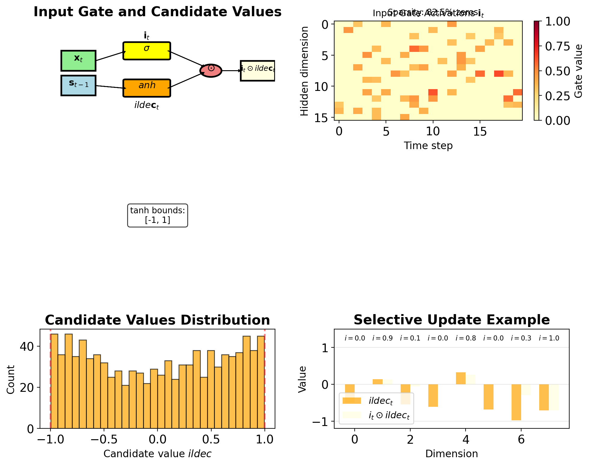
Input Gate Modulates New Information
Input gate (what to store): \[\mathbf{i}_t = \sigma(\mathbf{W}_i[\mathbf{s}_{t-1}, \mathbf{x}_t] + \mathbf{b}_i)\]
Candidate values (potential new content): \[\tilde{\mathbf{c}}_t = \tanh(\mathbf{W}_c[\mathbf{s}_{t-1}, \mathbf{x}_t] + \mathbf{b}_c)\]
Combined update: \[\mathbf{c}_t^{\text{new}} = \mathbf{i}_t \odot \tilde{\mathbf{c}}_t\]
Complete cell update: \[\mathbf{c}_t = \mathbf{f}_t \odot \mathbf{c}_{t-1} + \mathbf{i}_t \odot \tilde{\mathbf{c}}_t\]
Design choices:
- Input gate: Controls amount of update
- Candidate: Provides content of update
- Separation allows selective writing
Learned behavior (task-dependent):
- Input gates can learn selective update patterns
- Candidates represent potential state changes
- Gate values emerge from training objectives
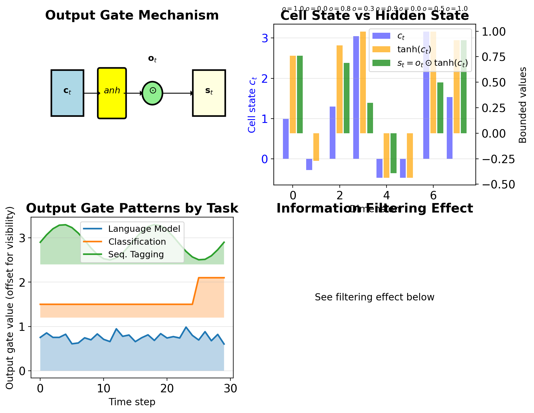
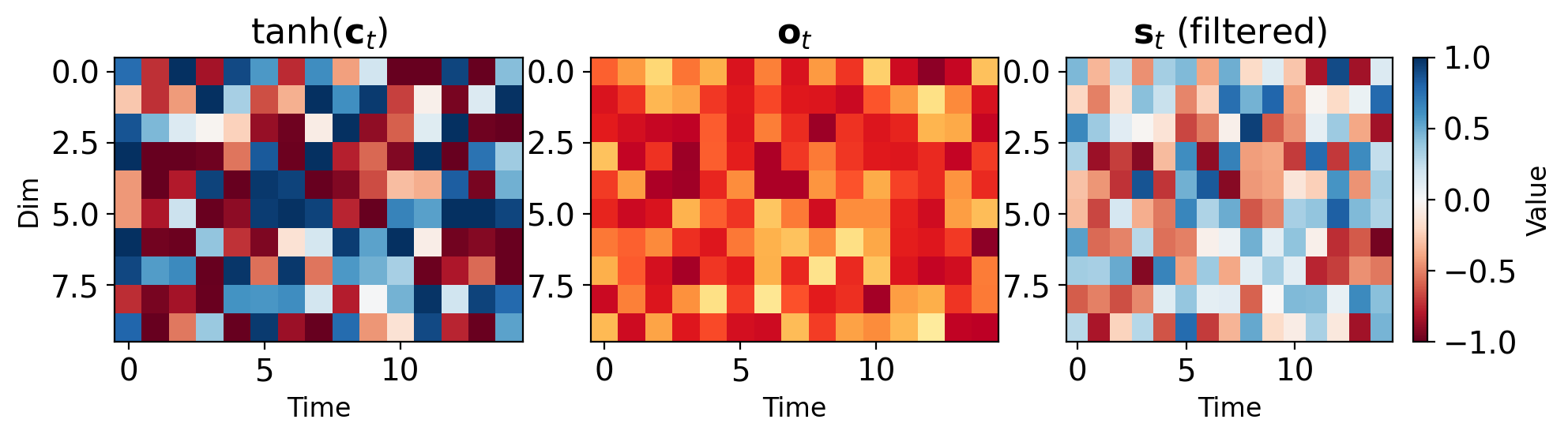
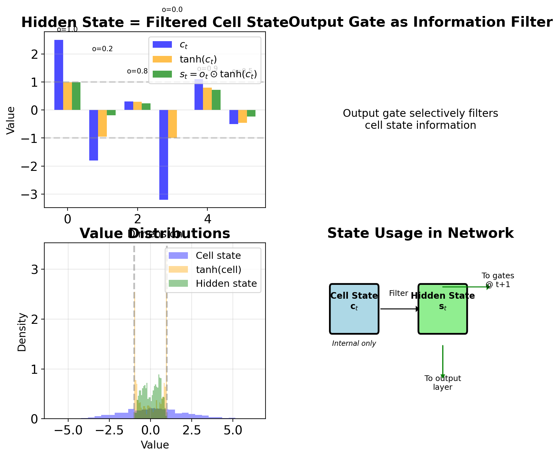
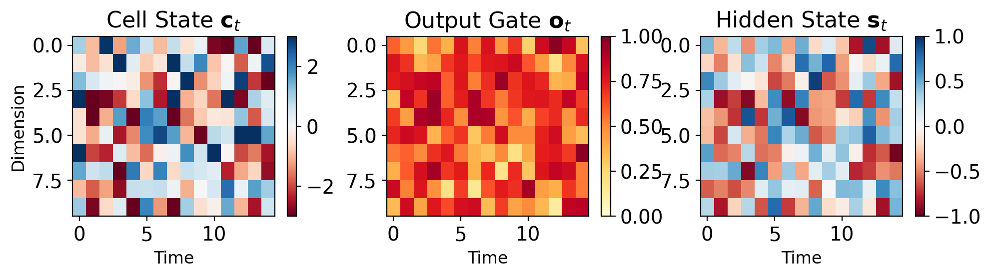
Output Gate Filters Cell State
\[\mathbf{o}_t = \sigma(\mathbf{W}_o[\mathbf{s}_{t-1}, \mathbf{x}_t] + \mathbf{b}_o)\]
Hidden state computation: \[\mathbf{s}_t = \mathbf{o}_t \odot \tanh(\mathbf{c}_t)\]
Design rationale:
- Cell state \(\mathbf{c}_t\) can grow unbounded
- \(\tanh(\mathbf{c}_t)\) bounds to [-1, 1]
- Output gate selects what to expose
Interpretation:
- Cell state: Complete internal memory
- Hidden state: Filtered working memory
- Output gate: Read controller
Task-dependent behavior:
- Language modeling: Often fully open
- Classification: Selective at decision points
- Sequence tagging: Varies by position
Dimension: Both \(\mathbf{o}_t, \mathbf{s}_t \in \mathbb{R}^H\)
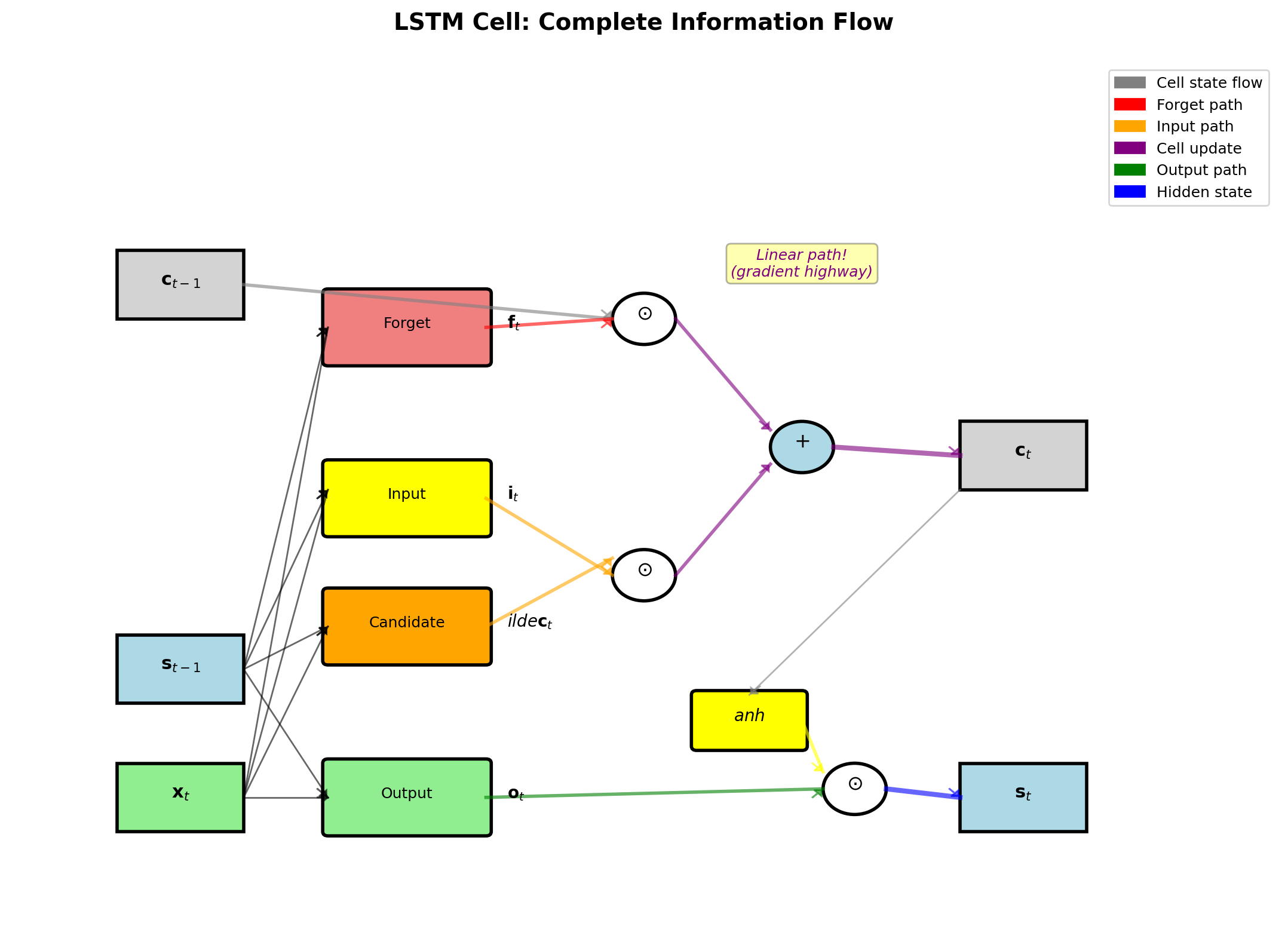
LSTM Gates Interact to Control Information Flow
Forget previous: \(\mathbf{f}_t \odot \mathbf{c}_{t-1}\)
Add new info: \(\mathbf{i}_t \odot \tilde{\mathbf{c}}_t\)
Update cell: \(\mathbf{c}_t = \mathbf{f}_t \odot \mathbf{c}_{t-1} + \mathbf{i}_t \odot \tilde{\mathbf{c}}_t\)
Output: \(\mathbf{s}_t = \mathbf{o}_t \odot \tanh(\mathbf{c}_t)\)
Parameter count:
- 4 weight matrices: \(\mathbf{W}_f, \mathbf{W}_i, \mathbf{W}_c, \mathbf{W}_o\)
- Each: \(H \times (H + D)\) dimensions
- Total: \(4H(H + D) + 4H\) parameters
- ~4× vanilla RNN parameters
Computational cost per timestep:
- 4 matrix multiplications
- 3 sigmoid, 2 tanh activations
- 5 element-wise operations
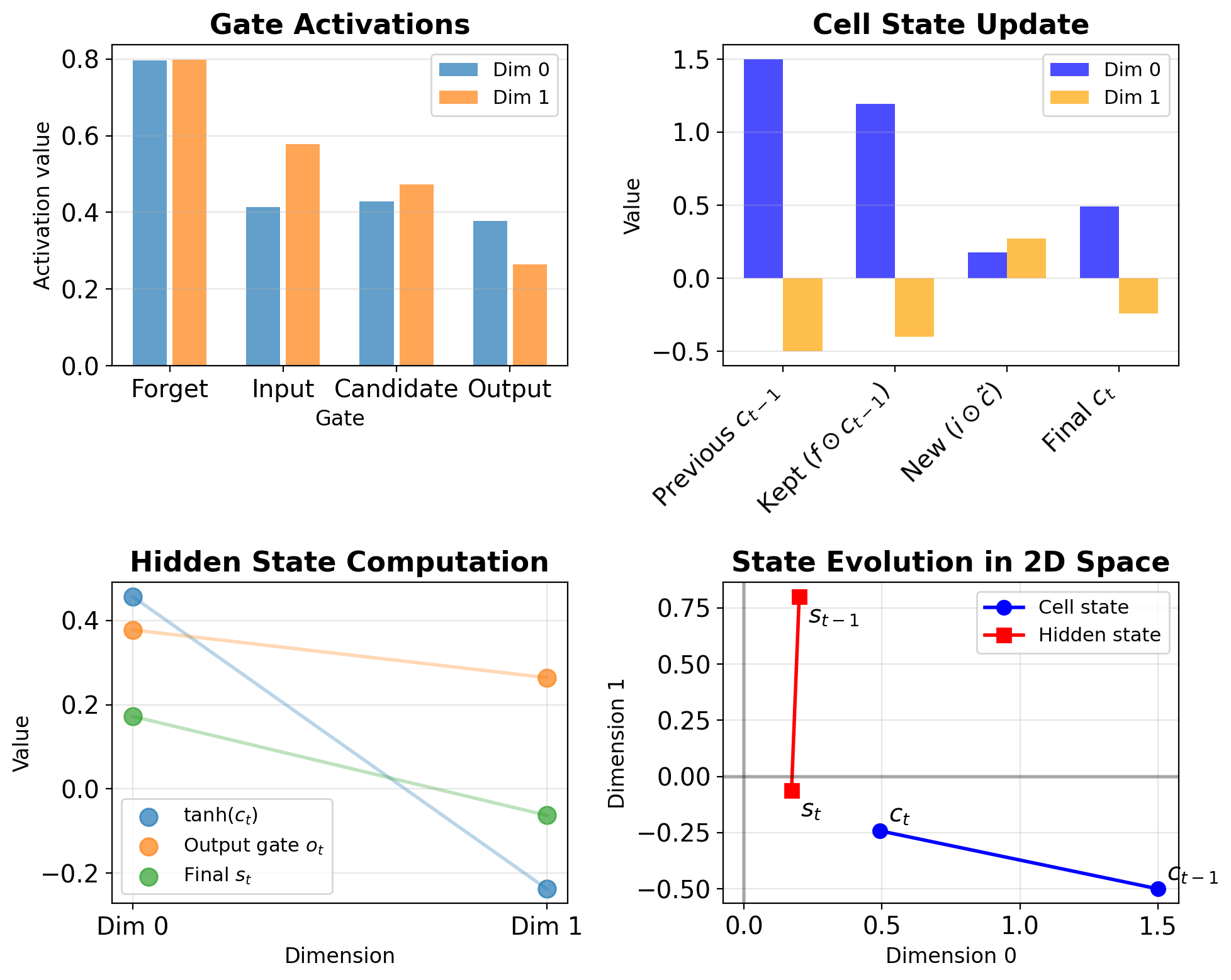
LSTM Operation on 2D Example
Given:
- Hidden size: \(H = 2\)
- Input size: \(D = 2\)
- Current input: \(\mathbf{x}_t = [0.5, -0.3]^T\)
- Previous hidden: \(\mathbf{s}_{t-1} = [0.2, 0.8]^T\)
- Previous cell: \(\mathbf{c}_{t-1} = [1.5, -0.5]^T\)
Step 1: Compute gates (simplified weights shown)
# Concatenate inputs
h_x = concat([s_t_1, x_t])  # [0.2, 0.8, 0.5, -0.3]

# Forget gate
f_t = sigmoid(W_f @ h_x + b_f)  # [0.9, 0.1]

# Input gate
i_t = sigmoid(W_i @ h_x + b_i)  # [0.2, 0.8]

# Candidate
c_tilde = tanh(W_c @ h_x + b_c) # [0.6, -0.4]

# Output gate
o_t = sigmoid(W_o @ h_x + b_o)  # [0.7, 0.5]
Step 2: Update cell state
c_t = f_t * c_t_1 + i_t * c_tilde
    = [0.9, 0.1] * [1.5, -0.5] + [0.2, 0.8] * [0.6, -0.4]
    = [1.35, -0.05] + [0.12, -0.32]
    = [1.47, -0.37]
Step 3: Compute hidden state
LSTM Cell State Update
\[\mathbf{c}_t = \mathbf{f}_t \odot \mathbf{c}_{t-1} + \mathbf{i}_t \odot \tilde{\mathbf{c}}_t\]
Components:
- \(\mathbf{f}_t \odot \mathbf{c}_{t-1}\): What to keep from past
- \(\mathbf{i}_t \odot \tilde{\mathbf{c}}_t\): What to add new
Improved gradient path:
- No activation function between \(\mathbf{c}_{t-1}\) and \(\mathbf{c}_t\)
- Gradient scaled by forget gate: \(\frac{\partial \mathbf{c}_t}{\partial \mathbf{c}_{t-1}} = \mathbf{f}_t\)
- Better preservation when \(\mathbf{f}_t \approx 1\)
Contrast with vanilla RNN:
- RNN: \(\mathbf{s}_t = \tanh(\mathbf{W}\mathbf{s}_{t-1} + ...)\)
- LSTM: \(\mathbf{c}_t = \mathbf{f}_t \odot \mathbf{c}_{t-1} + ...\)
- RNN forces through tanh every step
- LSTM can pass through unchanged
Cell state can grow unbounded:
- No activation function on \(\mathbf{c}_t\)
- Values can exceed [-1, 1]
- Controlled by output gate when read
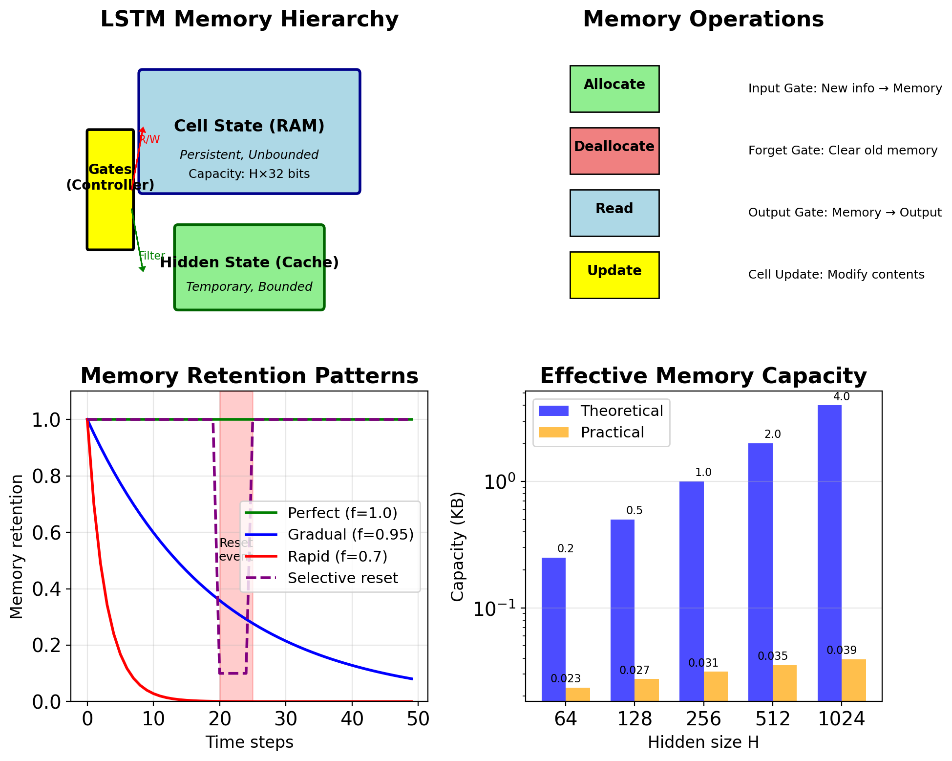
LSTM Cell State Resembles Computer Memory
Cell state = Long-term memory (RAM)
- Persistent storage across time
- Can hold information indefinitely
- Not directly observable
- Large capacity (unbounded values)
Hidden state = Working memory (Cache)
- Temporary, task-focused
- Bounded, normalized values
- Directly observable/usable
- Filtered view of long-term memory
Gates = Memory controller
- Forget gate: Memory deallocation
- Input gate: Memory allocation
- Output gate: Memory read operation
Capacity analysis:
- Theoretical: \(H\) floating point numbers
- Practical: Limited by gate dynamics
- Forget gate ≈ 1: Very long memory
- Forget gate ≈ 0: No memory
Memory access patterns:
- Content-based (gates depend on input)
- Learned, not hand-designed
- Task-specific optimization
LSTM Has 4× Parameters of Vanilla RNN
Dimensions:
- Input: \(\mathbf{x}_t \in \mathbb{R}^D\)
- Hidden/Cell: \(\mathbf{s}_t, \mathbf{c}_t \in \mathbb{R}^H\)
- Gates: \(\mathbf{f}_t, \mathbf{i}_t, \mathbf{o}_t \in \mathbb{R}^H\)
- Candidate: \(\tilde{\mathbf{c}}_t \in \mathbb{R}^H\)
Weight matrices (4 gates):
- \(\mathbf{W}_f, \mathbf{W}_i, \mathbf{W}_c, \mathbf{W}_o\)
- Each: \(\mathbb{R}^{H \times (H+D)}\)
- Bias: \(\mathbf{b}_f, \mathbf{b}_i, \mathbf{b}_c, \mathbf{b}_o \in \mathbb{R}^H\)
Total parameters: \[N = 4 \times [H \times (H + D) + H] = 4H(H + D + 1)\]
Example (typical NLP):
- \(D = 300\) (embedding), \(H = 512\)
- Params: \(4 \times 512 \times (512 + 300 + 1)\)
- = 1,664,512 ≈ 1.66M parameters
- Vanilla RNN: 416,256 ≈ 0.42M
- LSTM has ~4× parameters
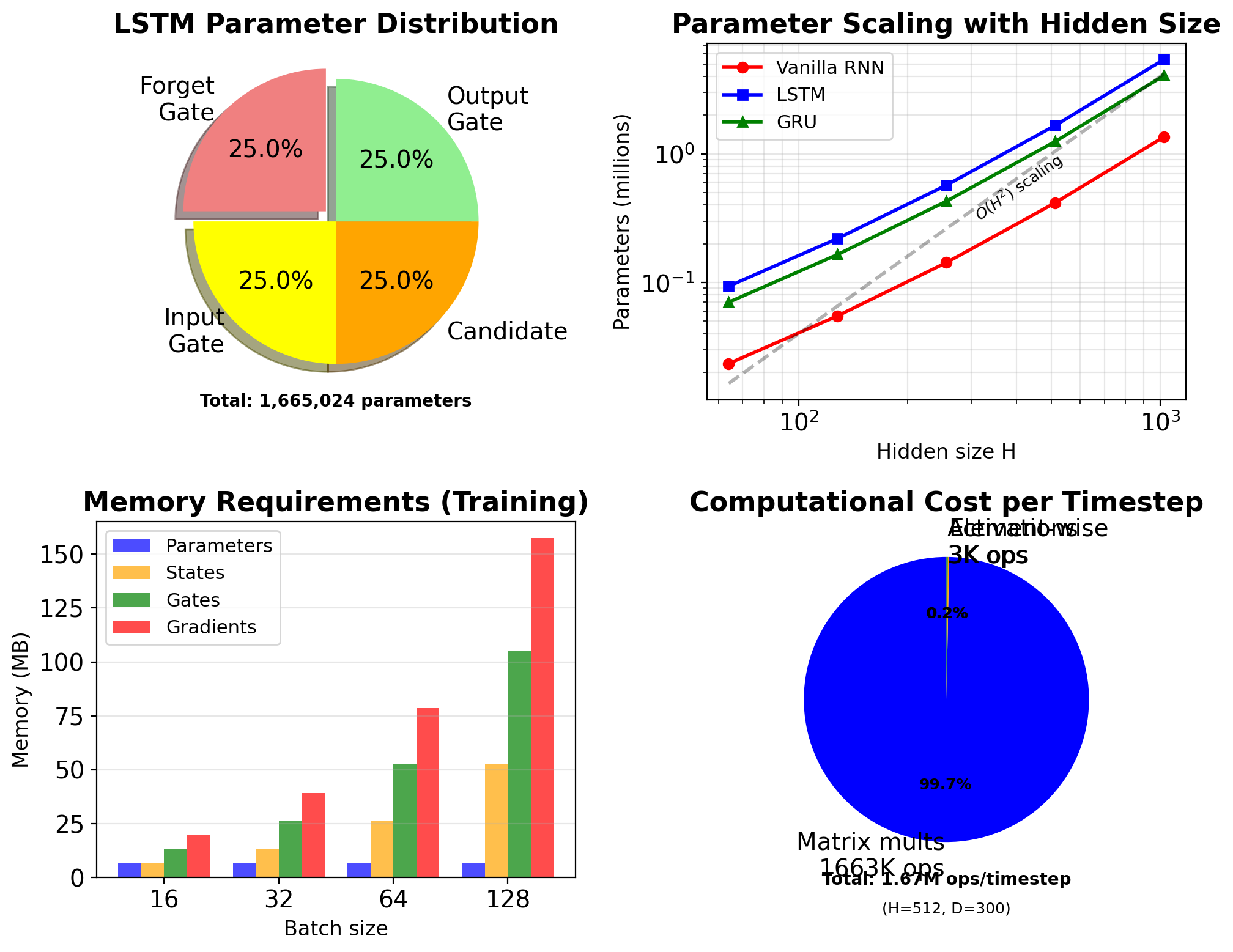
Matrix Operations Dominate LSTM Computation
Gate computations (f, i, o, g): \[4 \times [H(H + D) + H] = 4H(H + D + 1)\]
Cell state update: \[2H \text{ (element-wise ops)}\]
Hidden state: \[H \text{ (element-wise)}\]
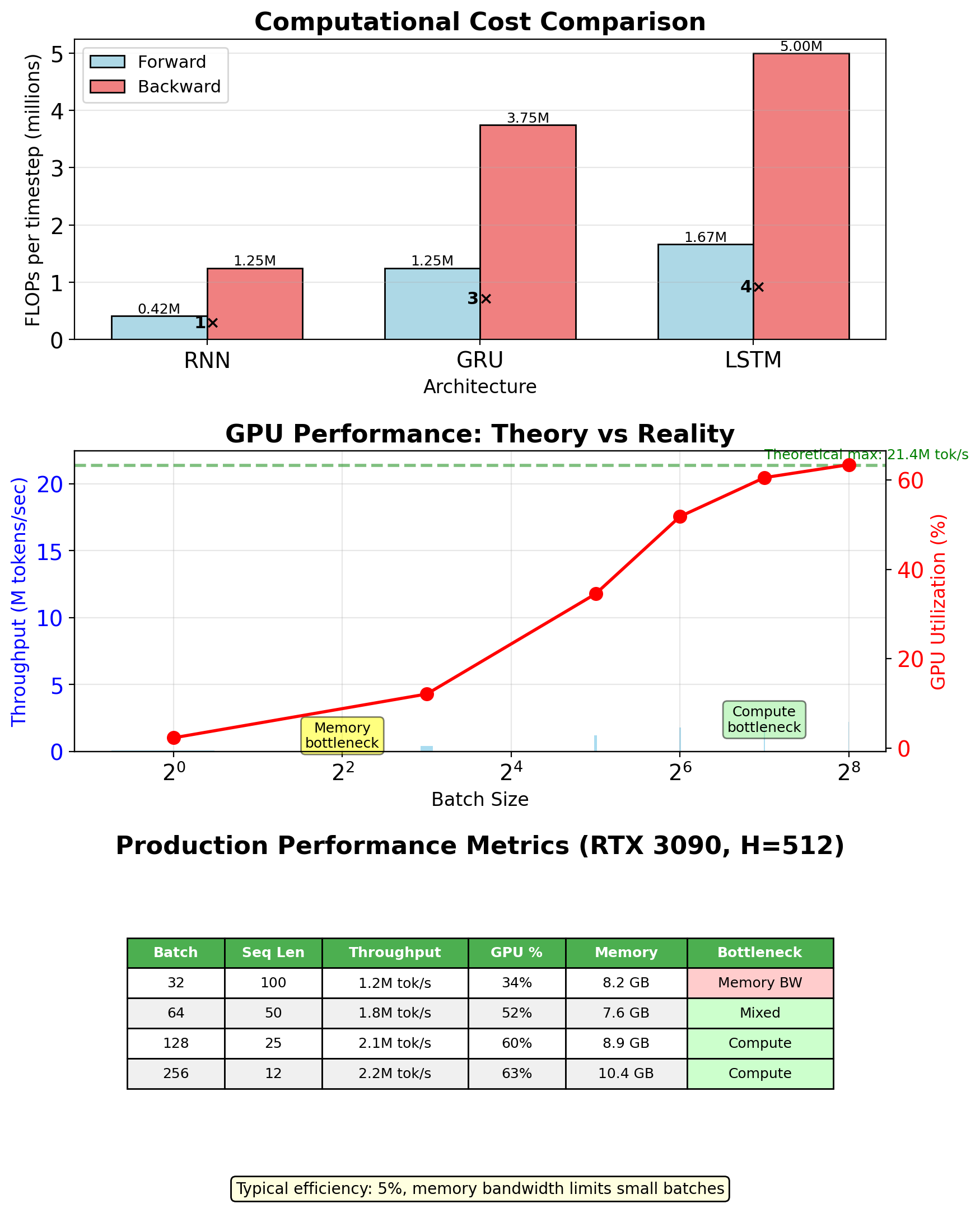
Total forward pass: \[\approx 4H(H + D + 1) \text{ FLOPs/timestep}\]
Backward pass (BPTT): \[\approx 12H(H + D + 1) \text{ FLOPs/timestep}\]
Comparison to vanilla RNN:
- RNN: \(H(H + D + 1)\) forward
- GRU: \(3H(H + D + 1)\) forward
- LSTM: \(4H(H + D + 1)\) forward
- 4× computational cost vs RNN
Matrix operations dominate:
- 99.3% matrix multiplications
- 0.7% element-wise operations
- Memory bandwidth is the primary bottleneck
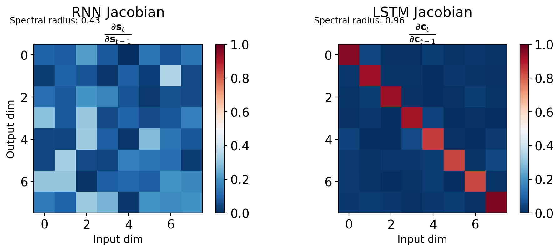
Cell State Creates Gradient Highway
Cell state gradient: \[\frac{\partial \mathbf{c}_t}{\partial \mathbf{c}_{t-1}} = \mathbf{f}_t\]
No nonlinearity - element-wise multiplication
Compare to vanilla RNN: \[\frac{\partial \mathbf{s}_t}{\partial \mathbf{s}_{t-1}} = \text{diag}(\tanh'(\mathbf{z}_t)) \cdot \mathbf{W}_{ss}\]
LSTM advantages:
- Linear path: No activation function between cell states
- Adaptive: Forget gate controls gradient flow
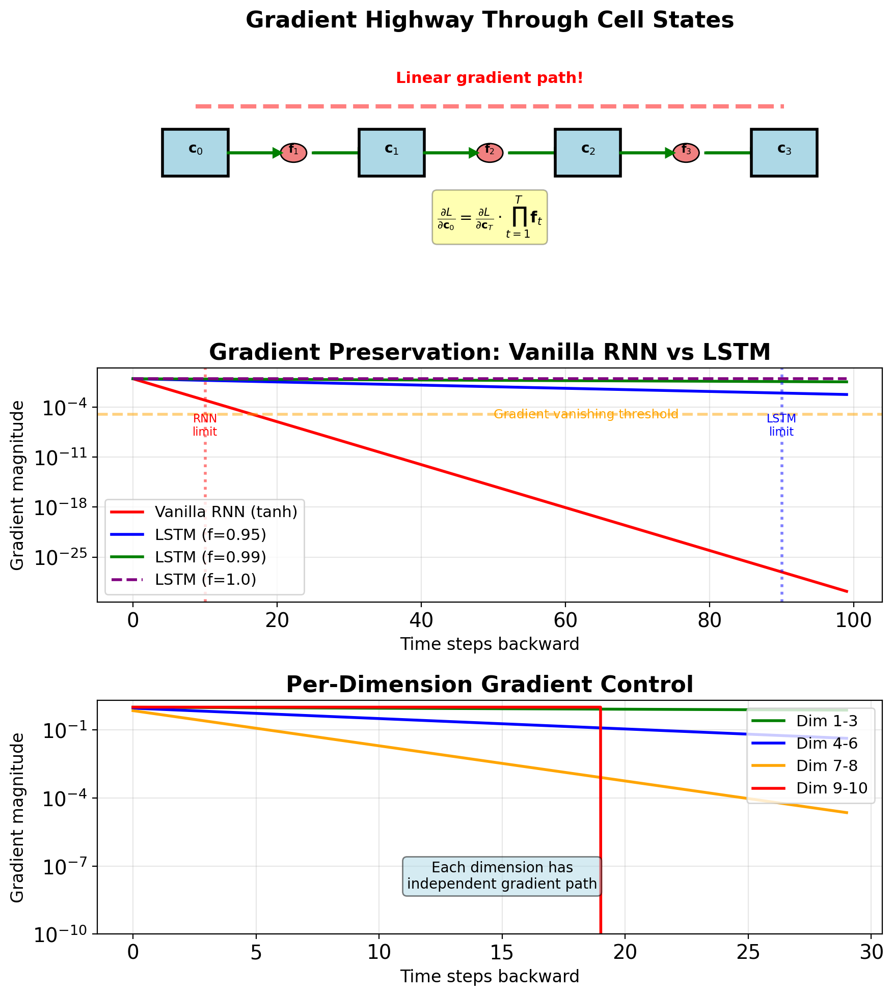
- Per-dimension: Each dimension has own gradient path
- Can preserve perfectly: If \(f_t = 1\), gradient passes unchanged
Long-term gradient: \[\frac{\partial \mathbf{c}_T}{\partial \mathbf{c}_0} = \prod_{t=1}^{T} \mathbf{f}_t\]
Element-wise product, not matrix product!
Gradient magnitude:
- If \(\mathbf{f}_t \approx 1\): Gradient preserved
- If \(\mathbf{f}_t \approx 0.9\): \(0.9^{100} \approx 10^{-5}\) (still vanishes)
- But much better than vanilla RNN!
Forget Gates Learn to Preserve Gradients
Initialization strategy:
- Bias \(b_f\) initialized to 1-2
- Results in initial \(f_t \approx 0.85-0.95\)
- Default: retain state, not discard
Learning progression:
Early training: High forget gates
- Preserve all information
- Allow gradient flow
Mid training: Selective forgetting
- Identify irrelevant information
- Task-specific patterns emerge
Late training: Refined gating
- Dimension-specific strategies
- Optimal memory-computation trade-off
Gradient contribution: \[\frac{\partial L}{\partial \mathbf{f}_t} = \frac{\partial L}{\partial \mathbf{c}_t} \odot \mathbf{c}_{t-1}\]
Gradient signal:
- Large gradient → high retention priority
- Small gradient → safe to forget

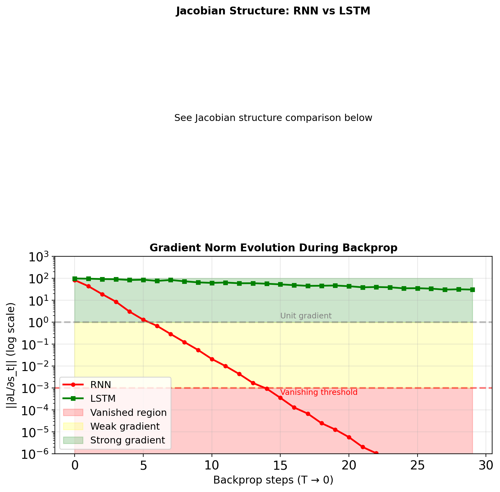
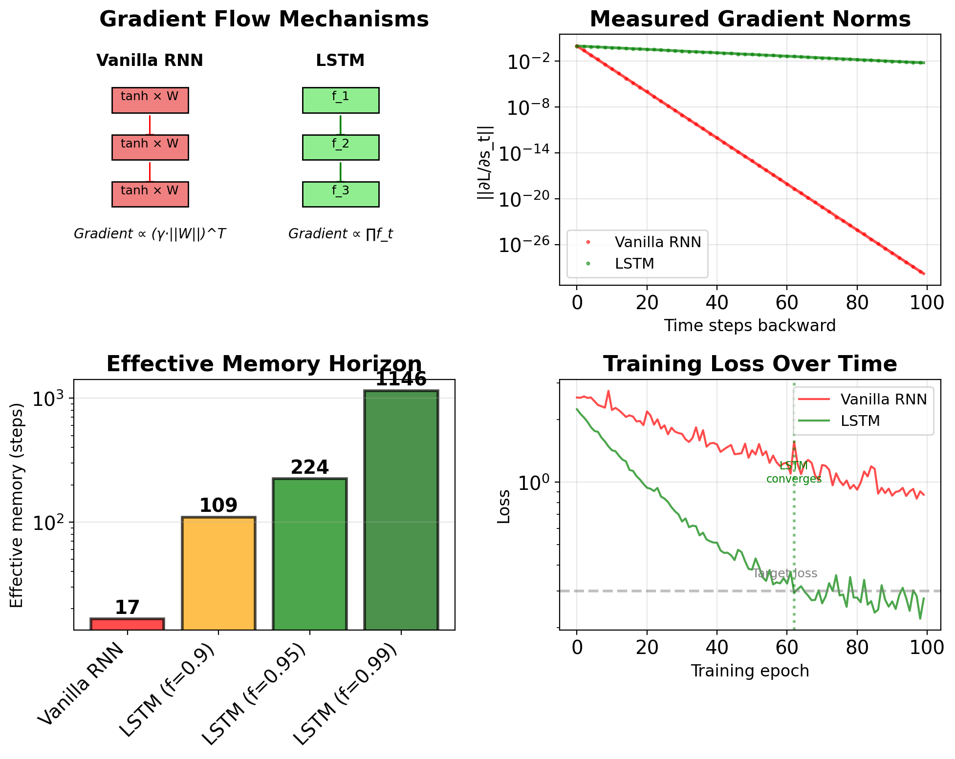
LSTMs Maintain Gradient Magnitude Better Than RNNs
Vanilla RNN gradient product: \[\prod_{t=k}^{T} \|\frac{\partial \mathbf{s}_t}{\partial \mathbf{s}_{t-1}}\| \leq \prod_{t=k}^{T} \gamma_{\text{tanh}} \cdot \|\mathbf{W}_{ss}\|\]
where \(\gamma_{\text{tanh}} \leq 1\) (≈ 0.5 in practice)
LSTM gradient product: \[\prod_{t=k}^{T} \|\frac{\partial \mathbf{c}_t}{\partial \mathbf{c}_{t-1}}\| = \prod_{t=k}^{T} \|\mathbf{f}_t\|\]
where \(\mathbf{f}_t \in [0,1]^H\) (0.9-0.95 in practice)
Comparing gradient flow:
- No weight matrix in LSTM path
- No repeated nonlinearity
- Adaptive per timestep
- Per-dimension control
Empirical measurements (Penn Treebank):
- Vanilla RNN: Gradient < 1e-5 after 10-15 steps
- LSTM: Gradient > 1e-5 up to 100+ steps
- 10× improvement in gradient preservation
LSTMs Extend Effective Memory Horizon
Definition: Distance where gradient > threshold \[\text{Horizon} = \max\{T : \|\frac{\partial L}{\partial \mathbf{s}_0}\| > \epsilon\}\]
\(\epsilon = 10^{-5}\) or \(10^{-6}\)
Analytical approximation:
- Vanilla RNN: \(T_{\text{eff}} \approx \frac{\log \epsilon}{\log \gamma}\)
- LSTM: \(T_{\text{eff}} \approx \frac{\log \epsilon}{\log \bar{f}}\)
where \(\bar{f}\) is average forget gate
Measured horizons (various tasks):
| Model | Horizon | Task |
|---|---|---|
| Vanilla RNN | 10-20 | Most tasks |
| LSTM (default) | 100-200 | Language modeling |
| LSTM (tuned) | 200-500 | Music generation |
| GRU | 80-150 | Translation |
Still has limits:
- Not infinite memory
- Degrades with depth
- Task-dependent effectiveness
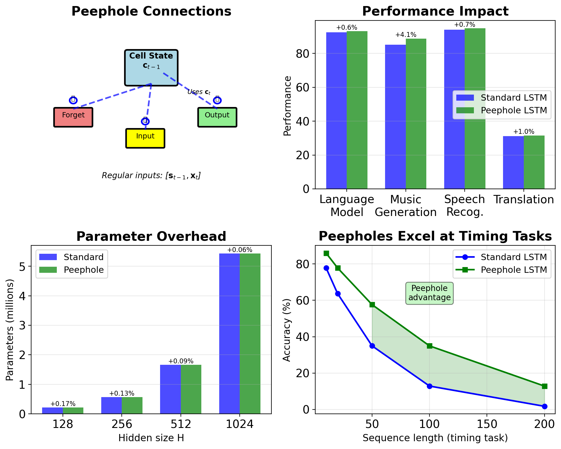
Peephole Connections Let Gates See Cell State
Standard LSTM gates: \[\mathbf{f}_t = \sigma(\mathbf{W}_f[\mathbf{s}_{t-1}, \mathbf{x}_t] + \mathbf{b}_f)\]
Peephole LSTM gates: \[\mathbf{f}_t = \sigma(\mathbf{W}_f[\mathbf{s}_{t-1}, \mathbf{x}_t] + \mathbf{P}_f \odot \mathbf{c}_{t-1} + \mathbf{b}_f)\]
All three gates get peepholes:
- Forget: uses \(\mathbf{c}_{t-1}\)
- Input: uses \(\mathbf{c}_{t-1}\)
- Output: uses \(\mathbf{c}_t\) (after update!)
Peephole weights:
- \(\mathbf{P}_f, \mathbf{P}_i, \mathbf{P}_o \in \mathbb{R}^H\)
- Diagonal matrices (element-wise)
- Adds 3H parameters total
Motivation:
- Gates see actual memory content
- Better for precise timing tasks
- Helps with counting/rhythm
Performance:
- Minor improvement (1-2%) on most tasks
- Improved performance on music/timing tasks
- Added complexity without commensurate gain
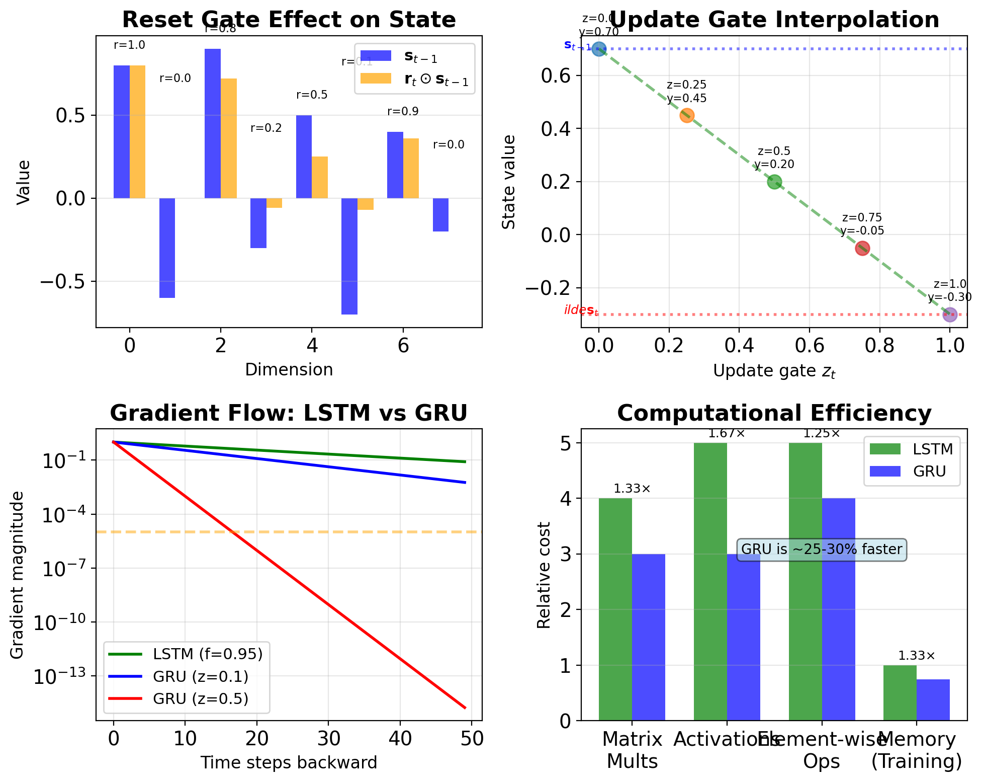
GRU Simplifies LSTM to Two Gates
GRU equations: \[\mathbf{z}_t = \sigma(\mathbf{W}_z[\mathbf{s}_{t-1}, \mathbf{x}_t] + \mathbf{b}_z)\] \[\mathbf{r}_t = \sigma(\mathbf{W}_r[\mathbf{s}_{t-1}, \mathbf{x}_t] + \mathbf{b}_r)\] \[\tilde{\mathbf{s}}_t = \tanh(\mathbf{W}[\mathbf{r}_t \odot \mathbf{s}_{t-1}, \mathbf{x}_t] + \mathbf{b})\] \[\mathbf{s}_t = (1-\mathbf{z}_t) \odot \mathbf{s}_{t-1} + \mathbf{z}_t \odot \tilde{\mathbf{s}}_t\]
Differences from LSTM:
- No separate cell state (c_t)
- Two gates instead of three
- Coupled forget/input via update gate z
- Reset gate modulates previous hidden state
Gate roles:
- Update gate z: How much to update (combines forget/input)
- Reset gate r: How much past to use for candidate
Advantages:
- 25% fewer parameters than LSTM
- Faster training/inference
- Often comparable performance
- Simpler to implement

Gradient Clipping Prevents Training Divergence
Norm clipping (standard approach): \[\mathbf{g}_{\text{clipped}} = \begin{cases} \mathbf{g} & \text{if } \|\mathbf{g}\|_2 \leq \theta \\ \theta \cdot \frac{\mathbf{g}}{\|\mathbf{g}\|_2} & \text{if } \|\mathbf{g}\|_2 > \theta \end{cases}\]
Implementation:
Starting points (tune based on gradient statistics):
- Small models: 1-5
- Seq2seq models: 5-10
- Deep networks: 10-25
Monitoring gradient statistics:
- Track percentage of batches clipped
- If >50% clipped: increase threshold
- If <1% clipped: consider decreasing for stability
Comparison with CNNs/Transformers:
- CNNs: Optional, rarely needed
- Transformers: Helpful but not required
- RNNs: Required - will diverge without it
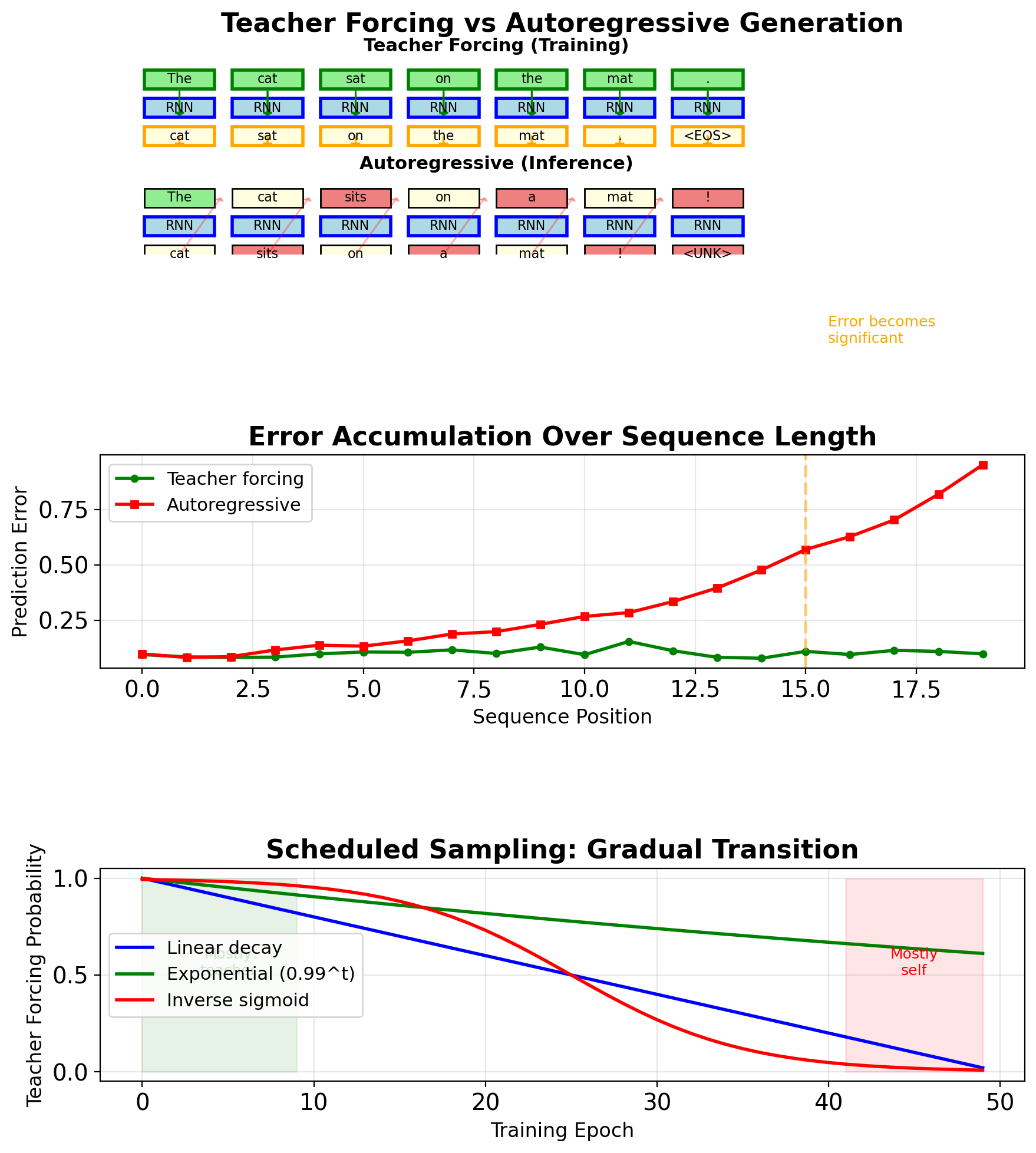
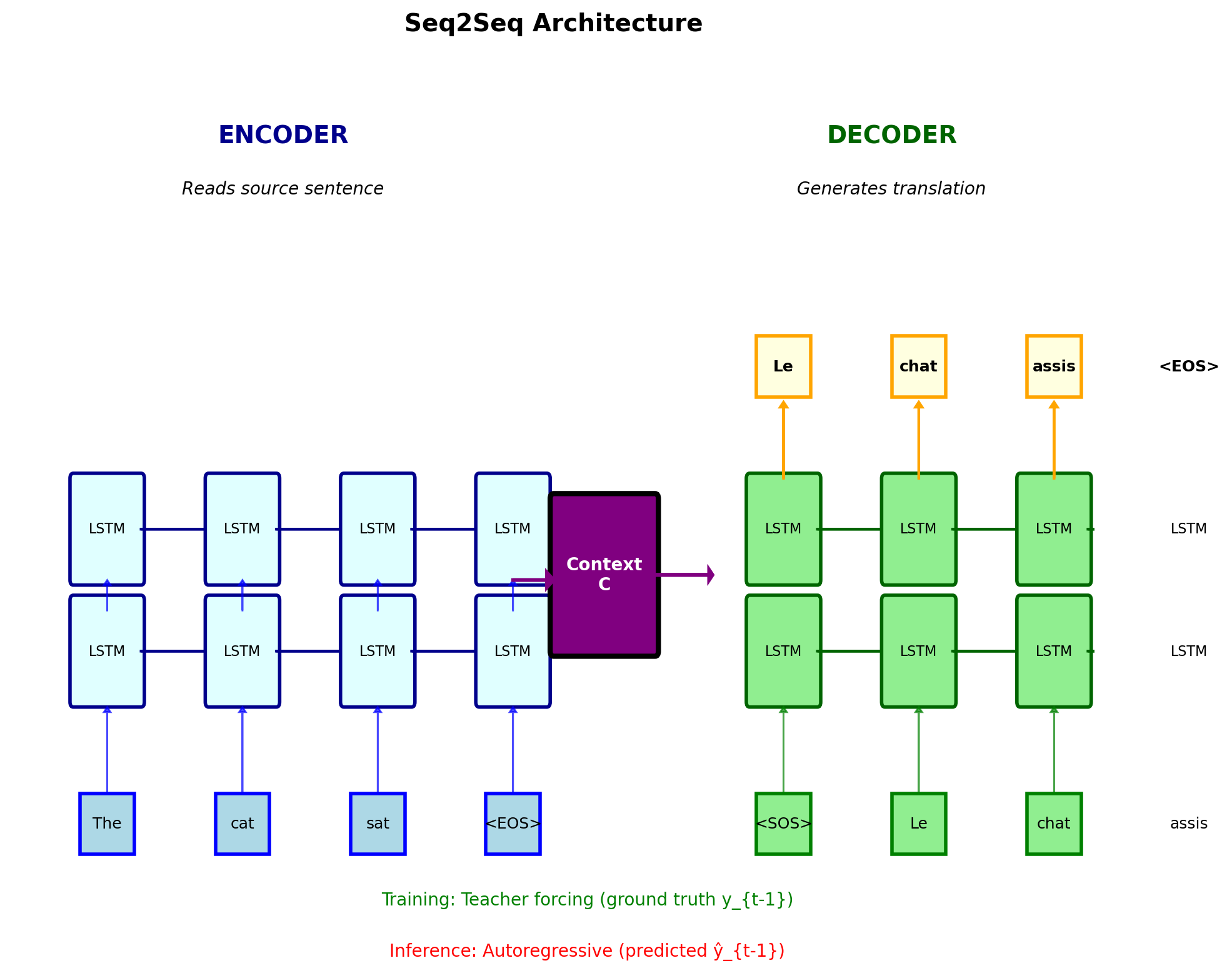
Teacher Forcing Creates Train-Test Mismatch
Training (Teacher Forcing):
- Input at t: ground truth \(y_{t-1}\)
- Model never sees its own errors
- Stable, fast convergence
- Loss: \(\mathcal{L} = \sum_t \ell(f(y_{t-1}), y_t)\)
Inference (Autoregressive):
- Input at t: prediction \(\hat{y}_{t-1}\)
- Errors compound over sequence
- No ground truth available
- Output: \(\hat{y}_t = f(\hat{y}_{t-1})\)
Exposure bias accumulation:
- Step 1: ε error
- Step 2: ε + δε error
- Step T: O(εT) error
Scheduled sampling solution:
- Probability of teacher forcing: \(p = k^i\)
- k = 0.95-0.99, i = epoch
- Gradually expose model to own predictions
- Trade-off: stability vs robustness
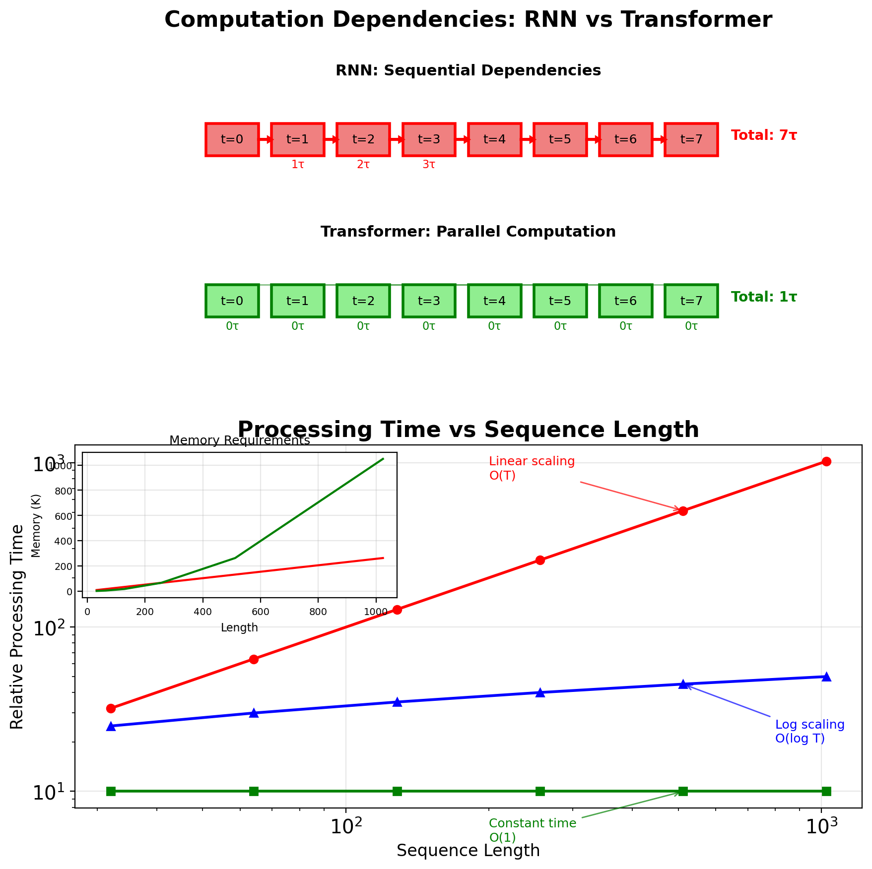
RNNs Cannot Parallelize Across Time Steps
Sequential dependency: \[\mathbf{h}_t = f(\mathbf{h}_{t-1}, \mathbf{x}_t)\]
Cannot compute \(\mathbf{h}_t\) without \(\mathbf{h}_{t-1}\)
Computational complexity:
- Per step: \(O(H^2)\) for hidden state update
- Total sequence: \(O(T \times H^2)\)
- Cannot parallelize across T
Memory requirements for BPTT:
- Store all hidden states: \(O(T \times H)\)
- Store all activations: \(O(T \times (D + H))\)
- Cannot discard until backward pass
Truncated BPTT trade-offs:
- Limit gradient flow to k steps
- Typical k = 20-35
- Memory: \(O(k \times H)\) instead of \(O(T \times H)\)
- Loses long-range gradients
Speed comparison (sequence length 512):
- RNN: 512 sequential operations
- CNN: log₂(512) = 9 with dilated convolutions
- Transformer: 1 operation (fully parallel)
This motivates attention mechanisms and transformers
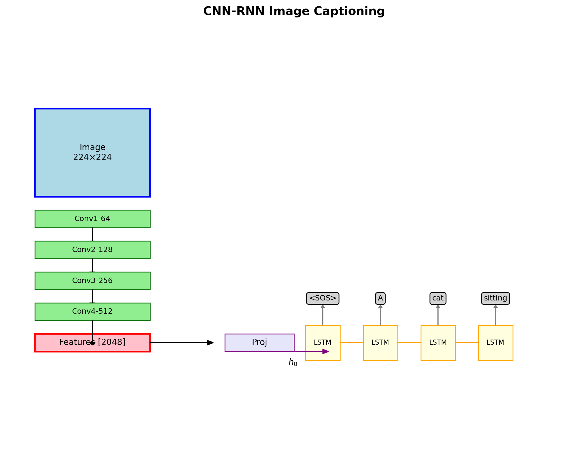
CNN-RNN Hybrids for Image Captioning
Components:
- CNN encoder
- ResNet-50/101 or VGG-16
- Output: \(\mathbf{v} \in \mathbb{R}^{2048}\)
- Pretrained weights frozen during training
- Linear projection
- \(\mathbf{h}_0 = \mathbf{W}_p \mathbf{v} + \mathbf{b}_p\)
- \(\mathbf{W}_p \in \mathbb{R}^{H \times 2048}\)
- LSTM decoder
- Hidden dimension: \(H = 512\)
- Vocabulary: \(|V| = 10,000\) tokens
- Teacher forcing ratio: 1.0 during training
Computational cost per image:
- CNN forward: 4.1 GFLOPs (ResNet-50)
- RNN decoding: 0.02 GFLOPs/word
- Total: ~4.5 GFLOPs per caption
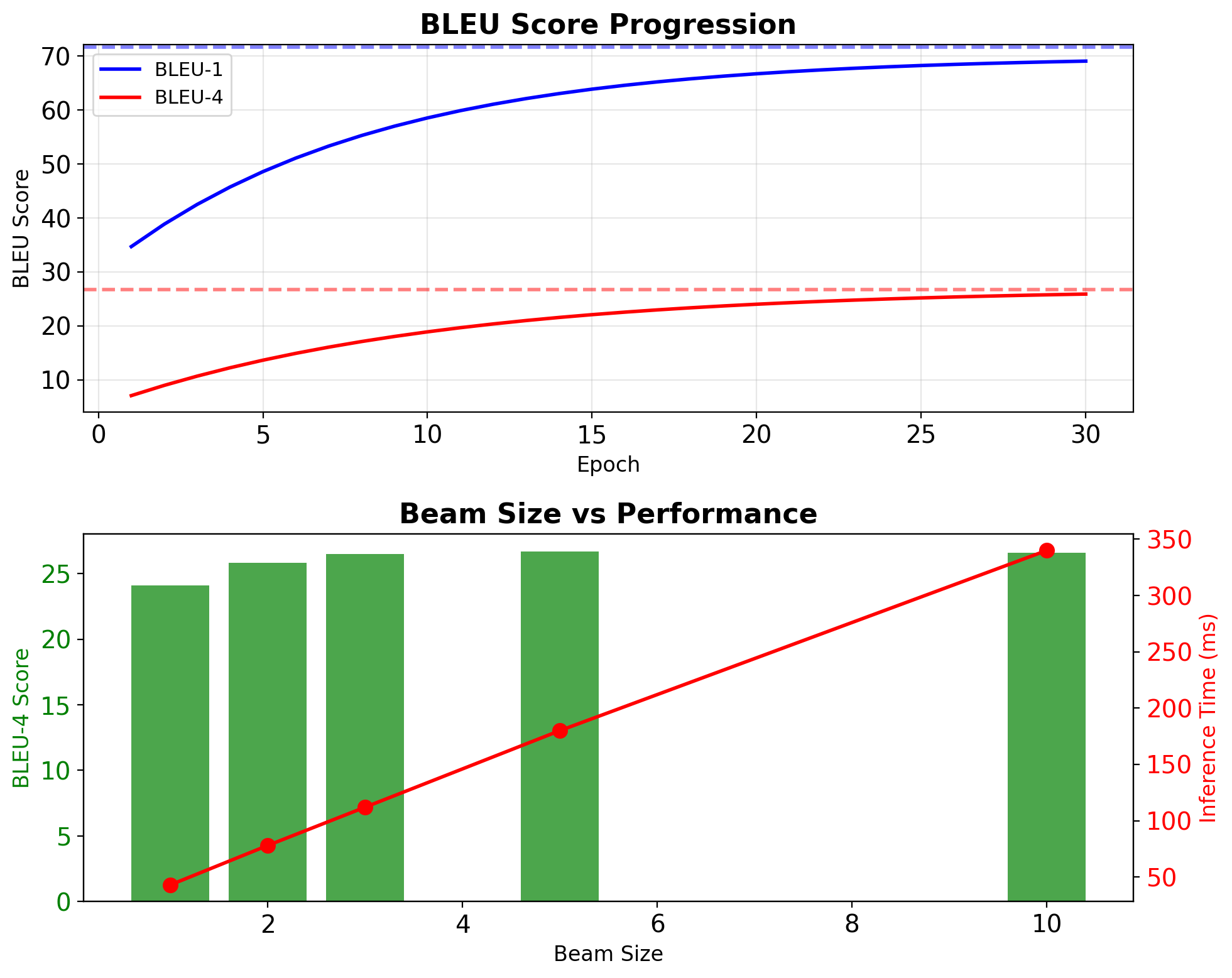
Hybrid Models Achieve Strong COCO Results
| Model | BLEU-1 | BLEU-4 | METEOR | CIDEr |
|---|---|---|---|---|
| CNN-RNN | 71.6 | 26.7 | 24.5 | 94.3 |
| + Attention | 74.1 | 31.5 | 26.0 | 107.2 |
| + Beam=5 | 72.8 | 28.9 | 25.2 | 98.1 |
Computational requirements:
- Memory: 8GB GPU for batch=32
- Training: 4.2 hours on V100 (30 epochs)
- Inference: 23 images/second
Failure modes:
- Hallucination: Non-existent objects in output
- Attribute binding: Color/property swapping
- Counting: Incorrect object quantities
- Exposure bias: Teacher forcing artifacts
Corrections:
- Scheduled sampling: \(p_{sample} = \min(0.5, \frac{epoch}{20})\)
- Length normalization: \(score_{norm} = \frac{score}{length^{0.6}}\)
- Diversity penalty: \(\lambda = 0.5\) for beam groups
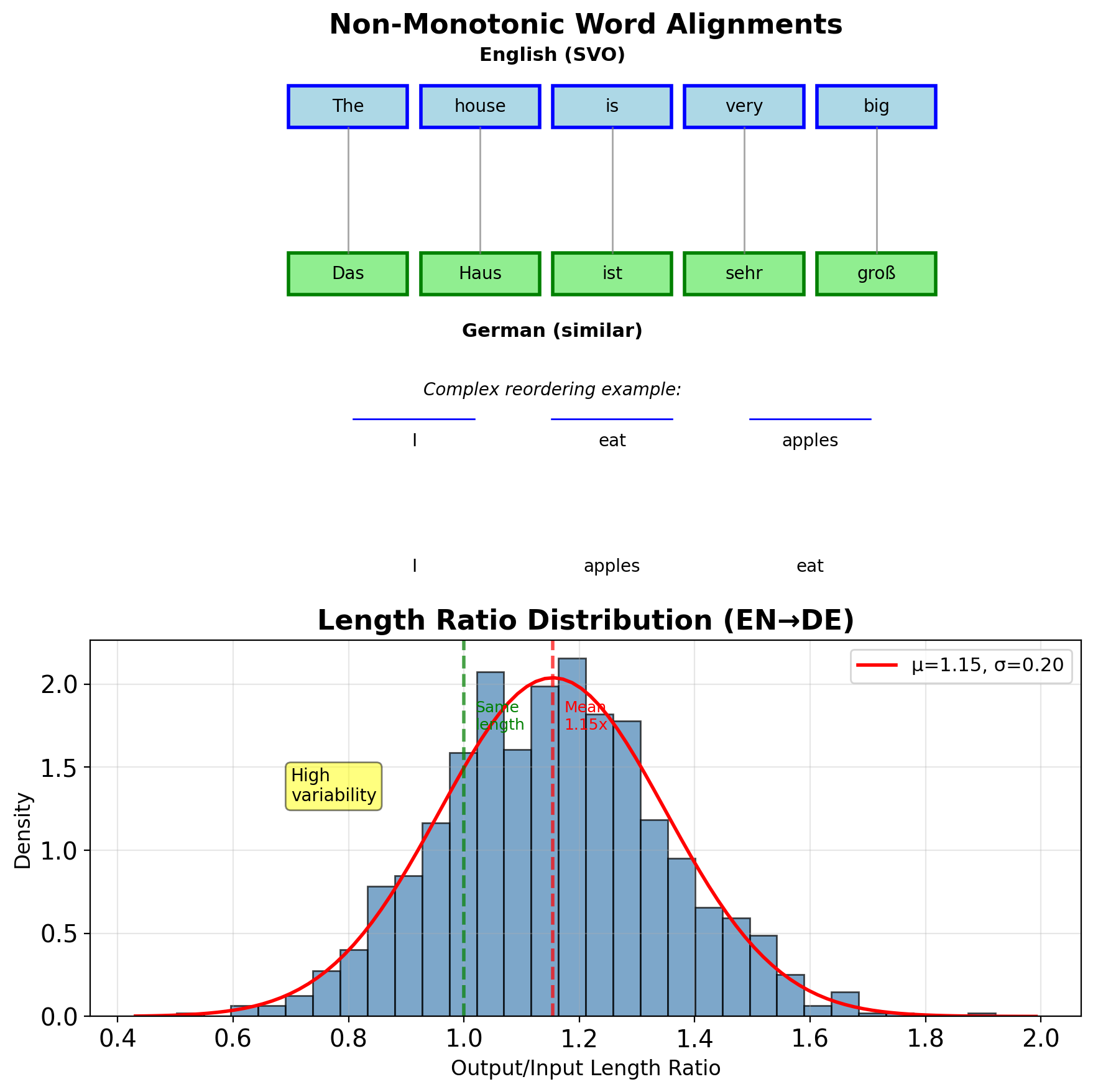
Translation Requires Variable-Length Mapping
- English: “The spirit is willing”
- Russian: “Дух бодр” (2 words)
- German: “Der Geist ist willig” (4 words)
- No fixed length relationship
Word order differences:
- English: Subject-Verb-Object (SVO)
- Japanese: Subject-Object-Verb (SOV)
- Arabic: Verb-Subject-Object (VSO)
- German: Verb-final in subordinate clauses
Non-monotonic alignment:
- “not” → “ne…pas” (French)
- “picked up” → “aufgehoben” (German)
- Phrasal verbs split across sentence
Statistical MT limitations:
- Phrase tables: Exponential combinations
- Feature engineering: Hand-crafted rules
- Pipeline components: Each adds errors
- No end-to-end optimization
BLEU Measures N-Gram Precision
\[p_n = \frac{\sum_{\text{n-gram} \in \hat{y}} \min(\text{Count}(\text{n-gram}), \text{Count}_{\text{ref}}(\text{n-gram}))}{\sum_{\text{n-gram} \in \hat{y}} \text{Count}(\text{n-gram})}\]
Combined score: \[\text{BLEU} = BP \cdot \exp\left(\sum_{n=1}^4 w_n \log p_n\right)\]
where \(w_n = 1/4\) (uniform weights)
Brevity penalty: \[BP = \begin{cases} 1 & \text{if } c > r \\ e^{1-r/c} & \text{if } c \leq r \end{cases}\]
- c = candidate length
- r = reference length
Typical scores:
- Human: 60-80
- Good system: 30-40
- Acceptable: 20-30
- Poor: <20

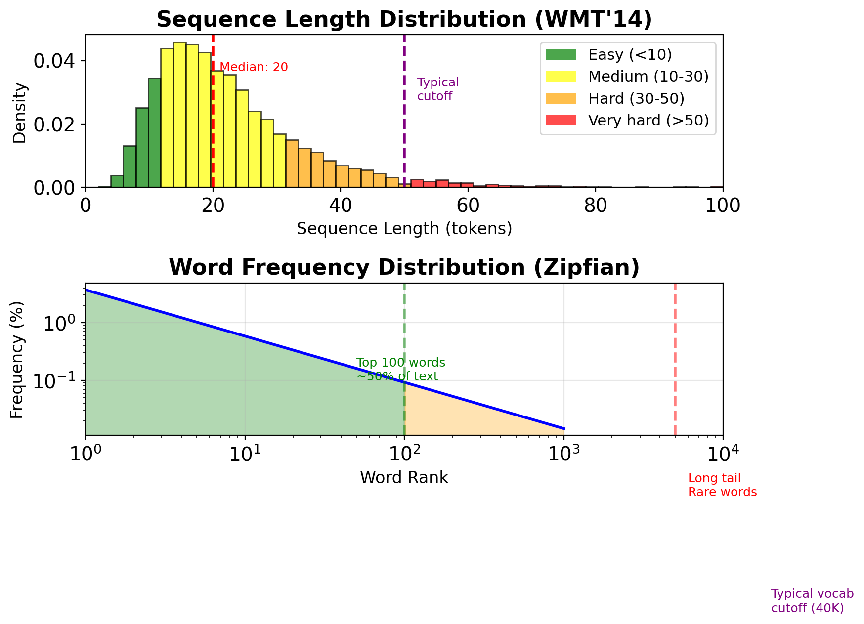
Modern NMT Requires Millions of Parallel Sentences
WMT’14 English-French dataset:
- 36M sentence pairs
- Average length: ~25 tokens
- Vocabulary: 40K (source), 40K (target)
- Total tokens: ~900M
Preprocessing challenges:
- Tokenization differences across languages
- Handling rare words (UNK token)
- Byte-pair encoding (BPE) for subwords
- Length filtering (remove >50 ratio outliers)
Computational requirements:
- Training time: Days to weeks on GPUs
- Memory: Storing all hidden states for BPTT
- Inference: Beam search multiplies computation
Data distribution issues:
- Zipfian word frequency
- Long tail of rare constructions
- Domain mismatch (news vs conversation)
- Evaluation set characteristics differ
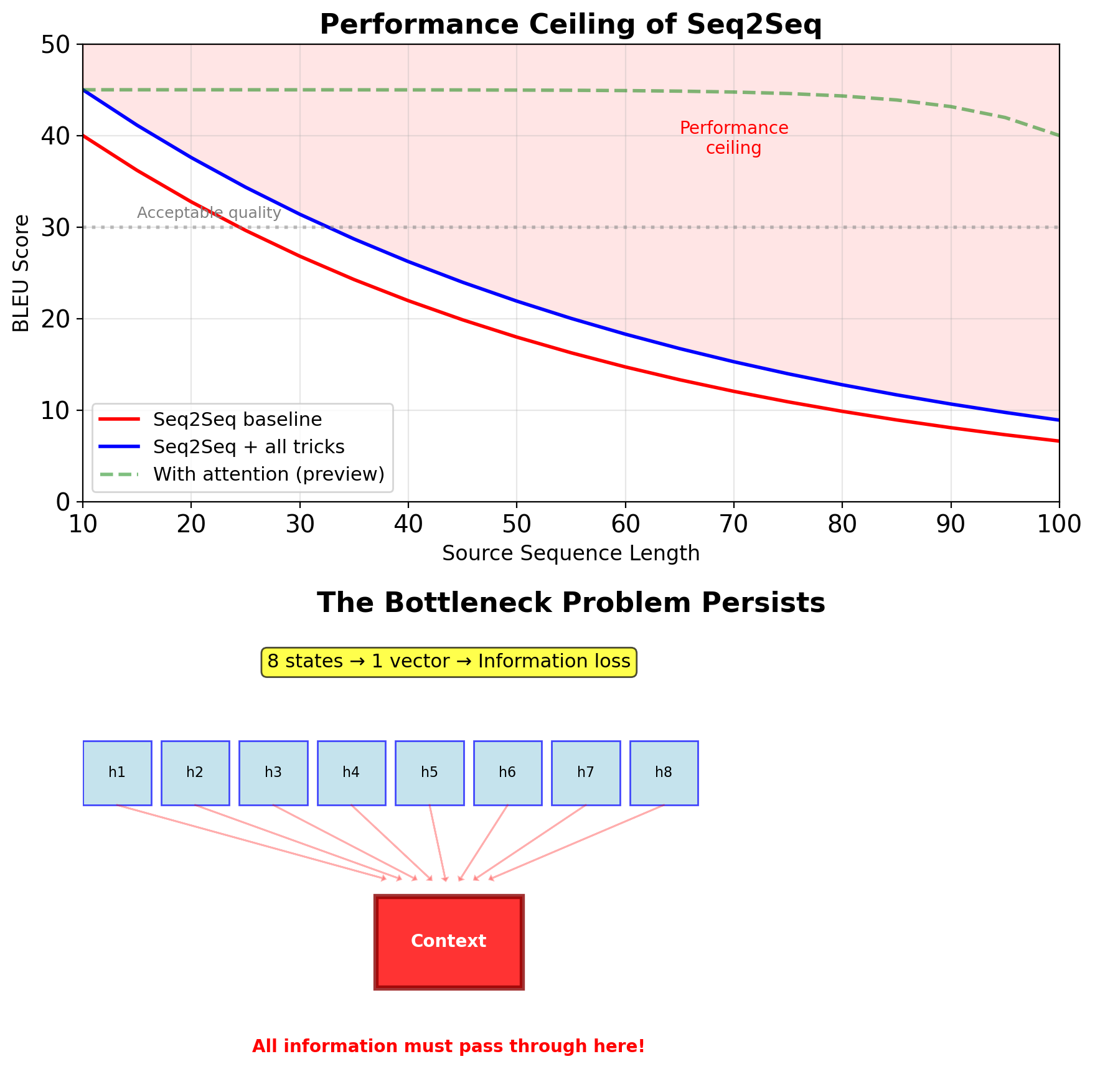
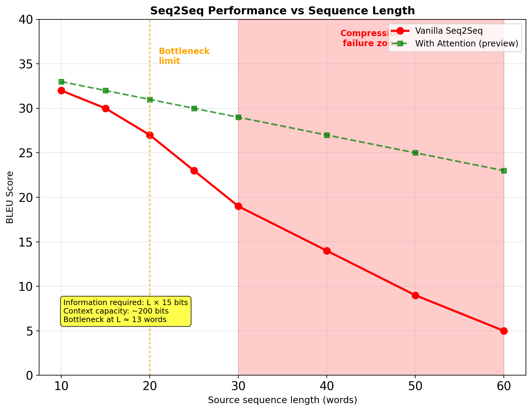
The Fixed-Size Bottleneck Problem
Variable-length sequences compressed to fixed H-dimensional vector:
- 10-word sentence → H dims
- 50-word sentence → H dims
- 100-word sentence → H dims
Information bottleneck problem:
- Upper bound: log₂(40K) ≈ 15 bits/word
- 50-word sentence: 750 bits theoretical max
- Context vector: H=1000 dimensions
- Severe information loss for long sequences
Observable failures:
- Performance degrades sharply after 15-20 words
- Later words overwrite earlier context
- Details are lost in compression
This motivates attention mechanisms (next lecture)
- Attention removes fixed-size constraint
- Each decoder step can access all encoder states
Encoder-Decoder Uses Two Separate RNNs
Encoder: Processes source sequence
- \(\mathbf{h}_t^{enc} = f_{enc}(\mathbf{h}_{t-1}^{enc}, \mathbf{x}_t)\)
- Final state: \(\mathbf{c} = \mathbf{h}_{T_{src}}^{enc}\)
Decoder: Generates target sequence
- Initialize: \(\mathbf{s}_0 = \mathbf{c}\)
- \(\mathbf{s}_t = f_{dec}(\mathbf{s}_{t-1}, \mathbf{y}_{t-1})\)
- \(P(\mathbf{y}_t | \mathbf{y}_{<t}, \mathbf{x}) = \text{softmax}(\mathbf{W}_o \mathbf{s}_t)\)
Standard configuration:
- LSTM for both encoder and decoder
- 2-4 layers deep
- Hidden size: 500-1000
- Vocabulary: 30K-50K tokens
- Special tokens:
, , ,
Training objective: \[\mathcal{L} = -\sum_{t=1}^{T_{tgt}} \log P(\mathbf{y}_t | \mathbf{y}_{<t}, \mathbf{x})\]
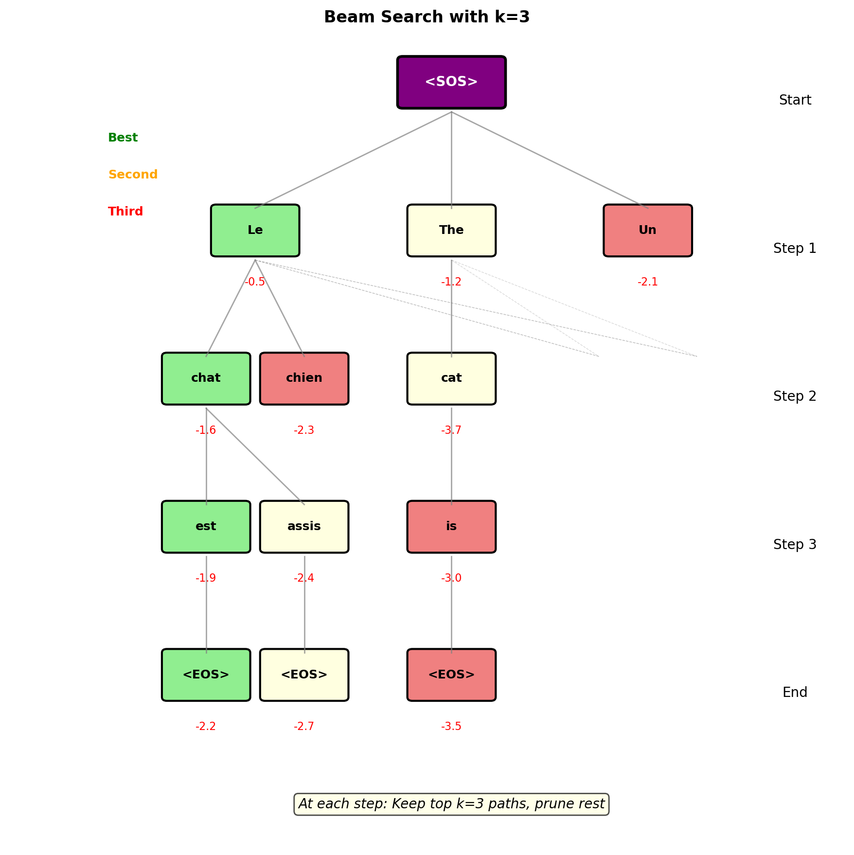
Beam Search Explores Multiple Hypotheses
- Beam width k: Number of hypotheses
- Cumulative log probability as score
- Exponential search space: V^T
- Beam search explores: k×T paths
Length normalization: \[\text{Score} = \frac{1}{L^\alpha} \sum_{t=1}^L \log P(y_t|y_{<t}, \mathbf{x})\]
Typical α = 0.6-0.7 (mild preference for longer)
Why log probabilities:
- Product of many P(y_t) → underflow
- Log turns product to sum
- Numerically stable
Beam search complexity:
- Time: O(k × V × T)
- Space: O(k × T)
- Trade-off: Quality vs speed
Input Reversal Improves Translation Quality
Discovery (Sutskever et al., 2014):
Reverse source sentence order
“A B C” → “C B A” → “X Y Z”
+2-4 BLEU improvement
Hypothesis: Reduces average path length
- First source word closer to first target
- Gradient flow improved for sentence beginnings
Deep architectures:
- 4-layer LSTM better than 2-layer
- Diminishing returns beyond 4
- Residual connections help beyond 4
Ensemble decoding:
- Train multiple models
- Average log probabilities
- +2-3 BLEU from 5-model ensemble
Results on WMT’14 En→Fr:
- Single model: BLEU ~30
- +Input reversal: BLEU ~33
- +Deep (4 layer): BLEU ~34
- +Ensemble: BLEU ~37
- State-of-art (2014): BLEU ~37

Fixed Context Vector Limits Seq2Seq
- Information compression inevitable
- Longer sequences → worse compression
- No direct path from source to target tokens
What seq2seq achieved:
- First end-to-end neural translation
- Competitive with phrase-based MT
- No feature engineering required
- Smooth optimization landscape
What it couldn’t solve:
- Sequences >50 tokens still fail
- Rare word handling (UNK problem)
- No alignment information
- Can’t revise earlier outputs
The bottleneck problem motivates attention:
- Allow decoder to look at all encoder states
- Dynamic, content-based addressing
- Soft alignment learned automatically
- Next lecture: Attention mechanisms