Sequence-to-Sequence Models

Sequences and Memory · Filters and State · The Recurrent Unit · Training Through the Loop · Gated Units · Recurrent Units as Components

Reading List

[Encoder-Decoder] K. Cho, B. van Merriënboer, C. Gulcehre, D. Bahdanau, F. Bougares, H. Schwenk, and Y. Bengio, “Learning phrase representations using RNN encoder–decoder for statistical machine translation,” in Proceedings of the 2014 Conference on Empirical Methods in Natural Language Processing, 2014, pp. 1724–1734.
[Seq2Seq] I. Sutskever, O. Vinyals, and Q. V. Le, “Sequence to sequence learning with neural networks,” in Advances in Neural Information Processing Systems, 2014, pp. 3104–3112.
[BLEU] K. Papineni, S. Roukos, T. Ward, and W.-J. Zhu, “BLEU: A method for automatic evaluation of machine translation,” in Proceedings of the 40th Annual Meeting of the Association for Computational Linguistics, 2002, pp. 311–318.
[Exposure] S. Bengio, O. Vinyals, N. Jaitly, and N. Shazeer, “Scheduled sampling for sequence prediction with recurrent neural networks,” in Advances in Neural Information Processing Systems, 2015, pp. 1171–1179.
[Decoding] P. Koehn and R. Knowles, “Six challenges for neural machine translation,” in Proceedings of the First Workshop on Neural Machine Translation, 2017, pp. 28–39.
[Length] K. Cho, B. van Merriënboer, D. Bahdanau, and Y. Bengio, “On the properties of neural machine translation: Encoder–decoder approaches,” in Proceedings of SSST-8, Eighth Workshop on Syntax, Semantics and Structure in Statistical Translation, 2014, pp. 103–111.
[Captioning] O. Vinyals, A. Toshev, S. Bengio, and D. Erhan, “Show and tell: A neural image caption generator,” in IEEE Conference on Computer Vision and Pattern Recognition, 2015, pp. 3156–3164.
[Alignment] D. Bahdanau, K. Cho, and Y. Bengio, “Neural machine translation by jointly learning to align and translate,” in International Conference on Learning Representations, 2015.

Translating a Sentence

Translations Have Their Own Length and Word Order

One pair, used throughout

“the black cat sat on the mat”, seven words
“le chat noir s’est assis sur le tapis”, eight words

Three mismatches in one sentence

Length: eight words for seven, and a different count for a different sentence
Order: “black cat” becomes “chat noir”, the adjective after the noun, so the correspondence lines cross
Count: “sat” becomes “s’est assis”, one word to two

Across languages

English, French, and German differ in where the verb and the adjective go, so crossings occur in most sentence pairs
No rule maps target position \(t\) to a source position: which source words a target word depends on varies from word to word

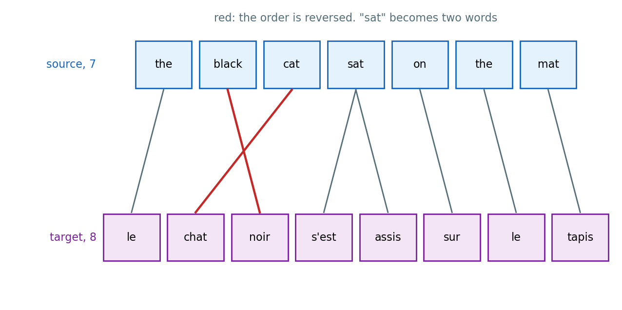
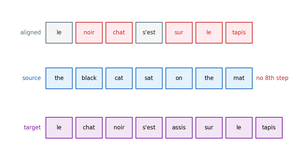
Outputs Aligned with the Source Cannot Produce a Translation

Outputs of a unit reading the source

One output per source word: seven outputs, in source order
One output for the sentence: one

Against the pair

Seven aligned outputs cannot hold eight words, and position 2 would hold “chat” where the source has “black”
A single output cannot hold a sentence

Required output

A sequence with its own length, set while it is produced
Each word a choice among a vocabulary of tens of thousands, in an order the target language sets
Words that agree with each other: “noir” is masculine because “chat” is

Translation Models Assign a Probability to Every Candidate Target

Object to build

\[p(\mathbf{y} \mid \mathbf{x}), \qquad \mathbf{x} = (x_1, \ldots, x_S),\ \mathbf{y} = (y_1, \ldots, y_T)\]

A distribution over target sentences, given the source
The set of candidates is every sequence of every length over the vocabulary: \(V^T\) sentences of length \(T\), \(40{,}000^{8} \approx 10^{37}\) for the example
No table can hold it. The model must be a function that scores any candidate it is given

Chain rule, exact

\[p(\mathbf{y} \mid \mathbf{x}) = \prod_{t=1}^{T} p(y_t \mid y_1, \ldots, y_{t-1}, \mathbf{x})\]

One factor per target word: a distribution over \(V\), conditioned on the source and on the target words already placed
No approximation in the factorization. What the model approximates is each factor

On the example

\(p(\text{le} \mid \mathbf{x}) \cdot p(\text{chat} \mid \text{le}, \mathbf{x}) \cdot p(\text{noir} \mid \text{le chat}, \mathbf{x}) \cdots\)
The third factor gives “noir” given “le chat” and the whole source: the factor that has to know the adjective follows the noun

Two conditioning inputs in every factor

The source \(\mathbf{x}\): a sequence, the same one for every factor
The prefix \(y_{<t}\): a sequence that grows by one word per factor

Both are sequences of unbounded length

A fixed-size state computed from a sequence is what the recurrent unit provides, and each factor needs two of them

Factorization Gives a Reader and a Writer

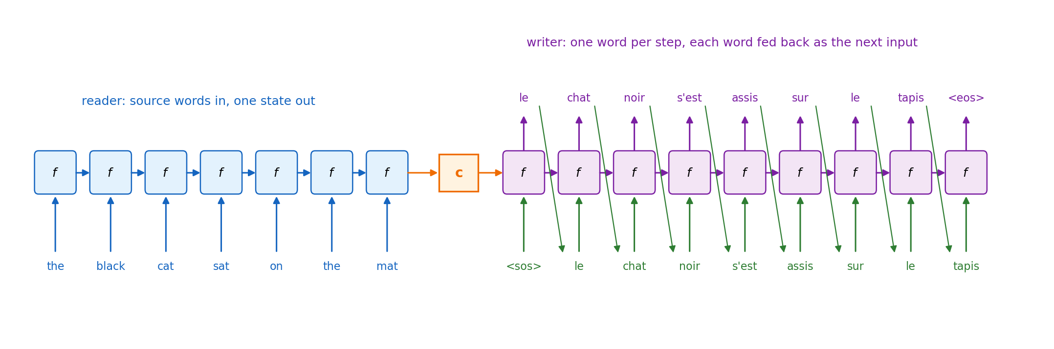
Reader

A recurrent unit takes \(x_1, \ldots, x_S\) and leaves one state, \(\mathbf{c} = \mathbf{h}^{\text{enc}}_S\)
\(\mathbf{c}\) is the only information about the source available to the rest of the model
The recurrent unit as built, used for its final state

Writer

A second recurrent unit starts from \(\mathbf{c}\) and produces one word per step
Its input at each step is the word it produced at the step before, so its state carries the prefix \(y_{<t}\)
Its readout at each step is the factor \(p(y_t \mid y_{<t}, \mathbf{x})\), and it stops when it emits the end token

Reading the source, writing the target, choosing the words at test time, and training the pair from data are the four parts of the model.

Sentence Pairs Are the Only Supervision

Parallel corpus

Pairs \((\mathbf{x}^{(n)}, \mathbf{y}^{(n)})\): a source sentence and one human translation of it
No word alignment, no marking of which target word came from which source word, no grammar
WMT’14 English-French: 36 million pairs from proceedings, news, and web text

Loss

\[L = -\sum_{n} \log p(\mathbf{y}^{(n)} \mid \mathbf{x}^{(n)}) = -\sum_{n}\sum_{t} \log p(y^{(n)}_t \mid y^{(n)}_{<t}, \mathbf{x}^{(n)})\]

The log-probability of the given translation under the model, and nothing else
One cross-entropy term per target word, so every word of every pair supplies a gradient

Not given

Which of the many correct translations is to be favoured: the corpus has one per source
Any signal at test time: a translation is produced without a reference to compare against

Scale

Vocabulary of tens of thousands of words on each side
Sentences of 20 to 30 words on average, up to 80 in the training data
Models of the size the reader and writer imply: two recurrent units, an embedding table on each side, a readout with \(V\) rows

BLEU Scores Translations by N-gram Overlap with References

Precision of each n-gram order

\[p_n = \frac{\text{candidate } n\text{-grams also in the reference, each counted at most as often as it appears there}}{\text{candidate } n\text{-grams}}\]

Score

\[\text{BLEU} = \text{BP} \cdot \exp\!\left(\tfrac{1}{4}\sum_{n=1}^{4} \log p_n\right), \qquad \text{BP} = \min\!\left(1,\ e^{\,1 - r/c}\right)\]

A geometric mean of the four precisions, reported from 0 to 100
\(c\) candidate length, \(r\) reference length: the brevity penalty, since precision alone rewards a short output
Computed over a whole test set, with n-gram counts pooled across sentences

Published anchors, WMT’14 English to French

Phrase-based baseline of the task: 33.3
Encoder-decoder, ensemble of 5: 34.8
Best system that year: 37.0

Against the reference “le chat noir s’est assis sur le tapis”

Candidate	\(p_1\)	\(p_2\)	\(p_3\)	\(p_4\)	BP	BLEU
le chat noir s’est assis sur le tapis	8/8	7/7	6/6	5/5	1	100
le chat noir est assis sur le tapis	7/8	5/7	3/6	1/5	1	50.0
le chat noir s’est	4/4	3/3	2/2	1/1	0.37	36.8
un chat noir était assis sur un tapis	5/8	2/7	0/6	0/5	1	0

One wrong word halves the score: it breaks every n-gram that contains it
A correct but incomplete output is held down by the brevity penalty alone
The last row is an acceptable translation (“a black cat was sitting on a mat”) and scores 0: no 3-gram matches the one reference

Limits

Matches surface words against one or a few references, so a valid rewording scores low
Unreliable for a single sentence. Its use is comparing systems over thousands of sentences
The standard machine-translation metric from 2002 through the first transformer results

Reading the Source

Reader Runs the Recurrent Unit for Its Final State

Reader

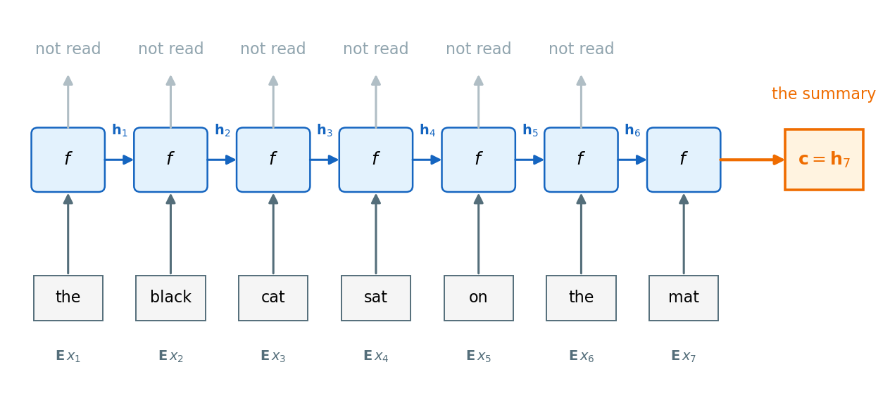
\[\mathbf{h}^{\text{enc}}_s = f\!\left(\mathbf{h}^{\text{enc}}_{s-1},\ \mathbf{E}\,x_s\right), \quad s = 1, \ldots, S, \qquad \mathbf{c} = \mathbf{h}^{\text{enc}}_S\]

\(\mathbf{E} \in \mathbb{R}^{V_{\text{src}} \times d}\): an embedding table, one learned \(d\)-vector per source word
\(f\): the recurrent unit, an LSTM in the published systems, so \(\mathbf{c}\) is the pair \((\mathbf{h}_S, \mathbf{C}_S)\)
No readout: the per-step states are computed and not used

Against tagging

The unit is run for one vector, not for its outputs
Its loss arrives from the writer, through \(\mathbf{c}\): the reader is trained to put in the summary what the writer’s loss rewards

Size

\(\mathbf{c} \in \mathbb{R}^H\), or \(2H\) numbers with the cell: \(H = 1000\) in the published system, for sentences of any length

Summary Must Carry the Whole Source

Writer’s input

\(\mathbf{c}\) and nothing else about the source: every content word, and their order, must be recoverable from it
\(H\) numbers for a sentence of \(S\) words: the same \(H\) at \(S = 6\) and \(S = 60\)

Memory demand

The first source word must survive \(S\) steps of the reader and then every step of the writer
The reader’s horizon is the recurrent unit’s horizon, and the same gradient has to reach the first step back through the whole source

Measured, with the writer’s inputs given

Teacher forcing removes the writer’s own errors, so what remains is what the summary carried
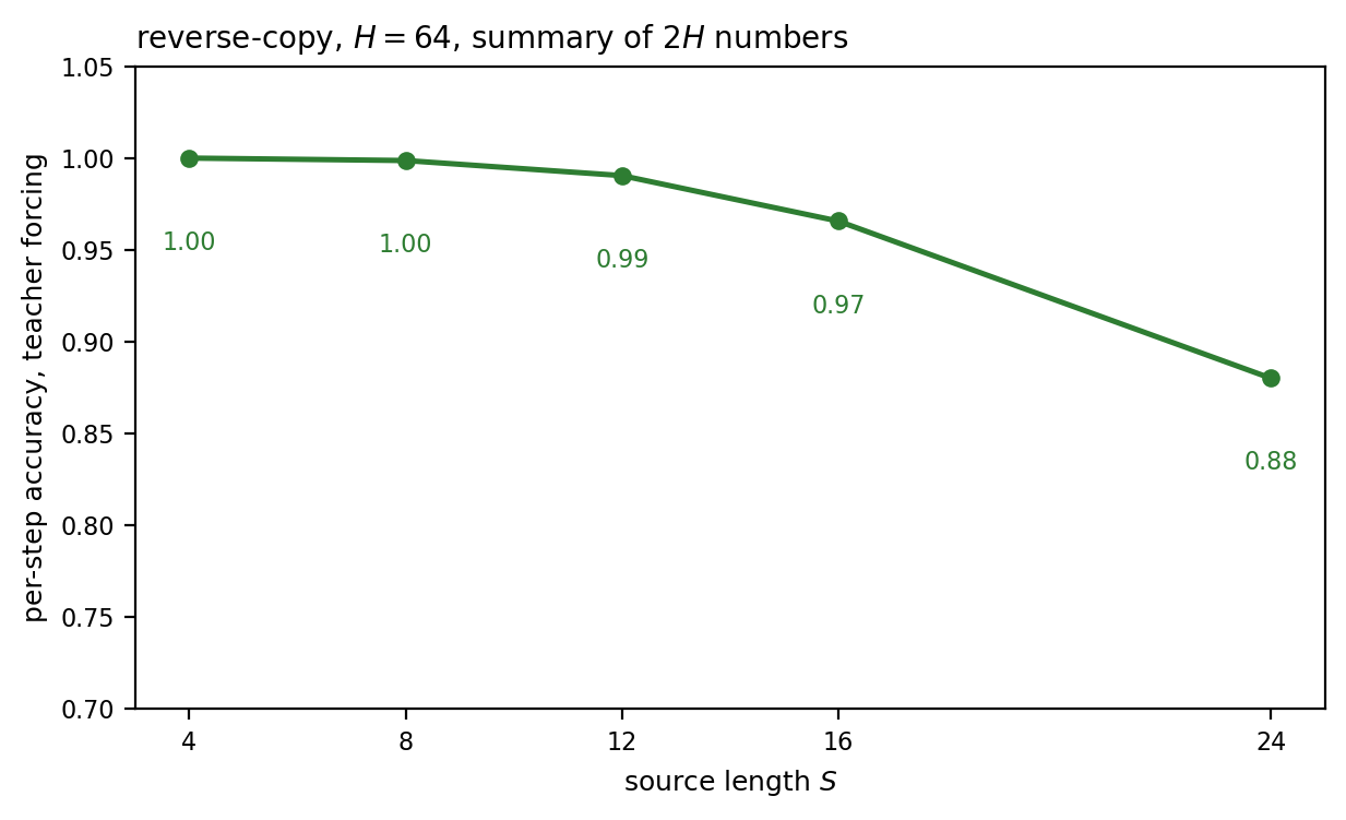
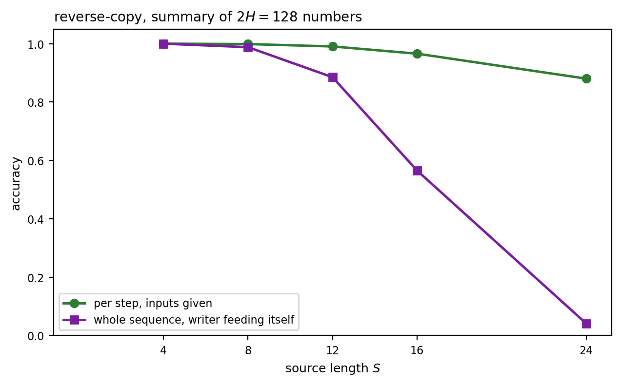
Per-step accuracy falls from 1.00 at \(T = 4\) to 0.88 at \(T = 24\) on the reverse-copy task

Reversing the Source Puts Its First Words Nearest the Writer

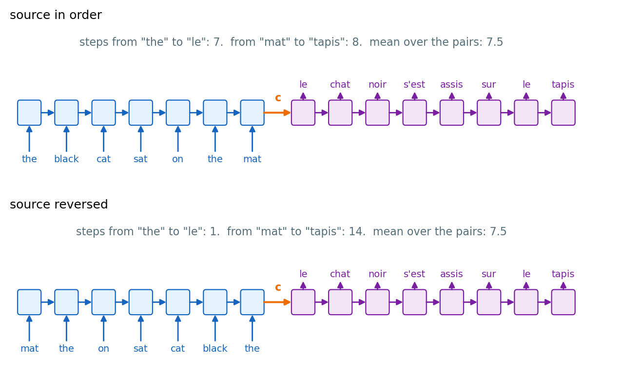
One change to the input

Feed the source words to the reader in reverse order and leave everything else as it is
The first source word is now the last read: one state step from \(\mathbf{c}\), and from the writer’s first word

Effect

The mean distance between a source word and its target word is unchanged
The minimum distance drops from \(S\) to \(1\): the writer’s first words, which decide the start of the sentence, are the ones with the shortest path
The gradient from the first target words reaches the first source words through a few steps instead of \(S\)

Published result

Sutskever et al. 2014, WMT’14 English to French, single model: BLEU 26.2 with the source in order, 30.6 reversed

Bidirectional Reader Ends One Step from Both Ends of the Source

Two readers, one summary

\[\overrightarrow{\mathbf{h}}_s = f_\rightarrow(\overrightarrow{\mathbf{h}}_{s-1}, \mathbf{E}x_s), \qquad \overleftarrow{\mathbf{h}}_s = f_\leftarrow(\overleftarrow{\mathbf{h}}_{s+1}, \mathbf{E}x_s)\]

\[\mathbf{c} = \left[\overrightarrow{\mathbf{h}}_S;\ \overleftarrow{\mathbf{h}}_1\right] \in \mathbb{R}^{2H}\]

The forward reader ends at the last word, the backward reader at the first
Each end of the source is one step from one half of the summary
Twice the reader’s parameters and compute, and the whole source must be available before reading starts, which translation allows

Unchanged

The summary is still one vector of fixed size, read once by the writer
A word in the middle of a long source is far from both ends
Every per-position state \(\overrightarrow{\mathbf{h}}_s, \overleftarrow{\mathbf{h}}_s\) is computed and then discarded, as in the one-directional reader

Keeping every state

Keeping all \(S\) pairs instead of the two ends is the design that gives the writer a position-wise view of the source, with weights from content

Non-Sequence Sources Need a Different Reader

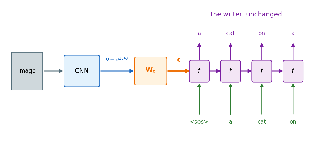
Captioning

The source is an image: no sequence to read, so no recurrent reader
A convolutional network trained for classification, with its classifier removed, gives one vector \(\mathbf{v}\) per image
A learned projection makes it the writer’s initial state: \(\mathbf{c} = \mathbf{W}_p \mathbf{v}\), \(\mathbf{W}_p \in \mathbb{R}^{H \times 2048}\)

Same writer, same training

The writer, the loss, and the sentence-pair supervision (image, caption) are the translation case’s
The convolutional network is kept fixed or fine-tuned, and the projection and the writer are trained from the captions

Summary

One vector for the whole image, read once: the same fixed-size summary, with the same limit

Writing the Target

Writer Is the Recurrent Unit with Its Output Fed Back

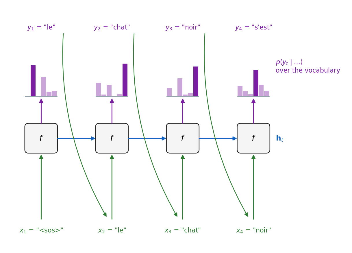
One step of the writer

Read the state out as a distribution over the target vocabulary: \(p(y_t \mid y_{<t}, \mathbf{x}) = \mathrm{softmax}(\mathbf{W}_{hy}\mathbf{h}_t + \mathbf{b}_y)\)
Choose one word from it
Feed the chosen word back as the next input, through the target embedding, and advance the state

One connection added to the recurrent unit

The recurrence and the readout as built, plus the connection from the chosen word to the next input
Through that connection \(\mathbf{h}_t\) depends on every word chosen so far, which is what each factor of the chain rule conditions on

Cost per word

One recurrence step and one readout: \(H(H + d) + V_{\text{tgt}} H\) multiply-adds, the readout dominant for a vocabulary of tens of thousands
Sequential by construction: word \(t + 1\) cannot be chosen before word \(t\)

Summary Enters the Writer Once or at Every Step

Once, as the initial state

\[\mathbf{h}_0 = \mathbf{c}, \qquad \mathbf{h}_t = f(\mathbf{h}_{t-1}, \mathbf{E}'y_{t-1})\]

The source enters at step zero and at no later step
Everything the writer holds about the source at step \(t\) has survived \(t\) steps of its own recurrence: the summary is one more thing the state must carry, alongside the prefix
The published English-French system (Sutskever et al. 2014)

At every step, as an input

\[\mathbf{h}_t = f\!\left(\mathbf{h}_{t-1}, [\mathbf{E}'y_{t-1};\ \mathbf{c}]\right)\]

\(\mathbf{c}\) is concatenated to the input at every step, and in the original form also to the readout
The source is re-read at every word, so the state carries only the prefix
The RNN encoder-decoder of Cho et al. 2014

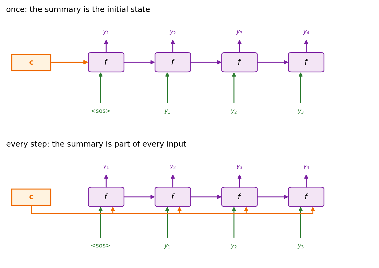
Same limit in both

One fixed-size vector stands for the whole source, however long, and the writer reads it as a whole

Training Feeds the Observed Target Word at Every Step

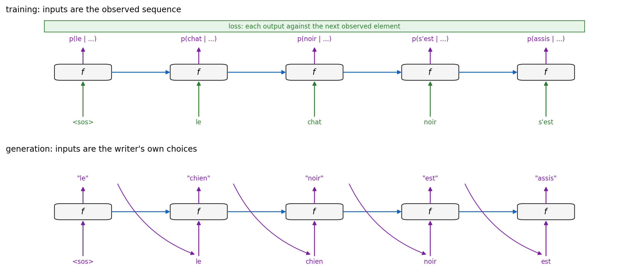
Teacher forcing

The target sentence is known in full, so the input at step \(t\) is \(y_{t-1}\) from the pair, regardless of the writer’s output at \(t - 1\)
All \(T\) inputs exist before the pass: one loop over the pair, one cross-entropy term per target word

\[L = -\sum_{t=1}^{T} \log p(y_t \mid y_{<t}, \mathbf{x})\]

Effect on the gradient

The gradient at each step is that of one classifier over \(V_{\text{tgt}}\), and it flows on through \(\mathbf{c}\) into the reader
Batches, padding, and truncation apply unchanged, since the loop receives a sequence of known inputs
Reported as perplexity, \(\exp(L / T)\): the effective number of equally likely words per step

One connection differs

Training: input from the pair. Generation: input from the writer. Every weight is shared between the two loops

One Wrong Word Changes Every Later Factor

Same writer, two prefixes

Step	Trained on (teacher forcing)	Generating, after one error
1	`<sos>`	`<sos>`
2	le	le
3	le chat	le chien
4	le chat noir	le chien noir
5	le chat noir s’est	le chien noir …

At step 2 the writer emits “chien” instead of “chat”: a probable word, the wrong one
Every later factor conditions on “le chien”, a prefix that appears in no training target for this source
The state now carries the writer’s own mistake, and the next choices are made from it

Exposure bias

In training the writer’s state has only ever followed correct prefixes, so its factors were fitted on those alone
At generation the inputs are its own choices, and the first error moves it to prefixes it was never scored on
Nothing in the loss measures how the writer behaves after its own error

Longer outputs, more exposure

Each output word is one more chance to leave the training prefixes
A sentence of thirty words is thirty chances, a paragraph hundreds: the gap between training and generation grows with the length of what is produced

Same mechanism wherever a model generates

Any model trained with teacher forcing and run on its own outputs: translation, captioning, speech synthesis, language models

Per-Word Errors Compound over the Sentence

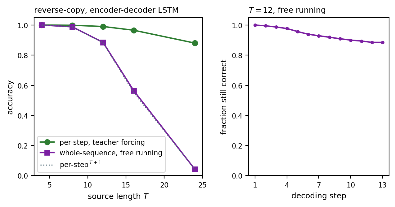
Measured

Reverse-copy task, encoder-decoder LSTM with \(H = 64\), trained with teacher forcing
\(T = 24\): per-step accuracy 0.88 under teacher forcing, whole-sequence accuracy 0.04 when the writer feeds itself
\(0.88^{25} = 0.04\): the per-step accuracies multiply over the 25 outputs

Two treatments

In training: scheduled sampling feeds the writer its own choice instead of the observed word on a growing fraction of steps, so it is trained on some of the prefixes it will produce (Bengio et al. 2015)
At generation: keep more than one hypothesis open while choosing, so one wrong word does not determine the rest of the sentence

Start and End Tokens Bound the Target

Token	Where	Role
`<sos>`	first writer input	starts the loop with no word chosen yet
`<eos>`	last target word	the writer ends the sentence by emitting it
`<pad>`	after `<eos>` in a batch	fills shorter targets to the batch length, masked out of the loss

The target vocabulary gains the three tokens: \(V_{\text{tgt}} + 3\) rows in the readout and entries in \(\mathbf{E}'\)
<pad> is never predicted and never scored

Length set by the writer

Generation stops when <eos> is chosen, so the target length is not fixed in advance
A maximum length caps the loop if <eos> is never emitted
Every training target ends with <eos>, so emitting it at the right point is part of what is learned

On the example

Target: “le chat noir s’est assis sur le tapis ”, nine outputs for seven source words
A correct translation requires every word and the <eos> in place

Choosing the Words

Best Sentence Is Not the Sequence of Best Words

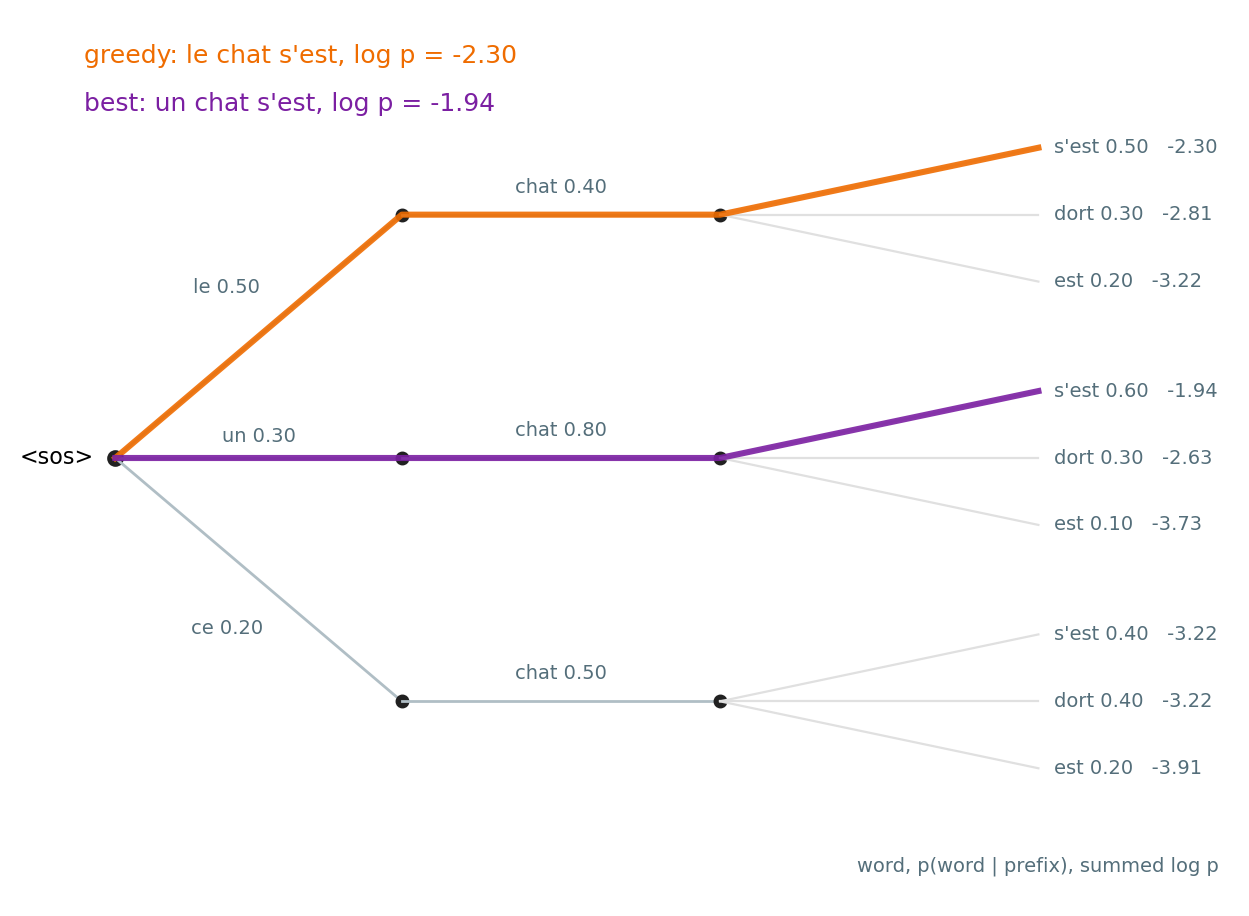
Test-time search

\[\hat{\mathbf{y}} = \arg\max_{\mathbf{y}} \prod_{t} p(y_t \mid y_{<t}, \mathbf{x}) = \arg\max_{\mathbf{y}} \sum_t \log p(y_t \mid y_{<t}, \mathbf{x})\]

The model scores any candidate. Finding the best one is a search over \(V^T\) candidates
The log turns the product into a sum, so each word adds a negative term to the score

No word can be chosen alone

The factor for word \(t\) conditions on the prefix: a probable first word can lead only to improbable continuations
In the tree, “le” is the most probable first word and “un chat s’est” is the most probable sentence
The exact maximum needs every path: \(V^T\) evaluations of the writer, out of reach for \(V\) in the tens of thousands

Greedy Decoding Takes the Most Probable Word at Each Step

state = encoder(src)                 # the summary c
word = SOS
out = []
while word != EOS and len(out) < max_len:
    logits, state = decoder(word, state)
    word = logits.argmax()           # the most probable next word
    out.append(word)

Cost

One writer step and one readout per output word: \(T\) steps for a sentence of \(T\) words
Memory: one state

Found

One path through the tree, the one that is locally best at every step
The score of that path is at most the best score, and the gap is not measured by the procedure

Missed

Any sentence whose first word is not the most probable first word
Any correction: a word, once chosen, is never revisited, and the prefix it creates is the only one the rest of the search considers

Beam Search Keeps \(k\) Hypotheses Open So a Worse Start Can Win

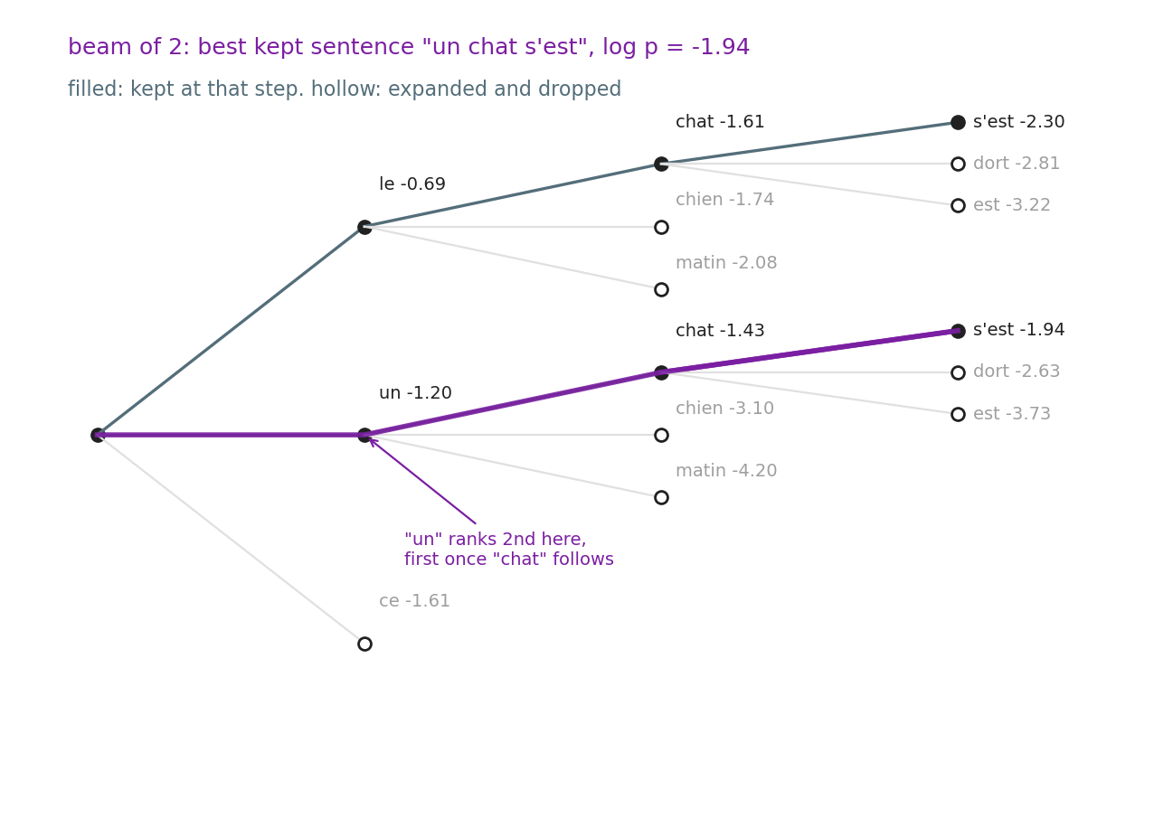
Hypotheses kept open

A hypothesis is a prefix with its summed log-probability. Keeping \(k\) of them lets a prefix that starts worse overtake one that starts better
In the tree, “un” is second after step 1 and leads after step 2, because \(p(\text{chat} \mid \text{un})\) is high

Procedure, width \(k\)

Start with one prefix, <sos>, score 0
Extend every kept prefix by every word: \(k \cdot V\) candidates, each scored by its summed log-probability
Keep the \(k\) best candidates
Repeat until every kept prefix has emitted <eos> or reached the maximum length, then return the best

Cost

\(k\) writer steps per output position, \(k \cdot V\) scores to sort: \(k\) times greedy in compute, and \(k\) states in memory
\(k = 1\) is greedy. \(k = V^T\) is the exact search

Found

The best sentence among those whose every prefix was in the top \(k\) at its step
A sentence can still be lost if one of its prefixes fell below \(k\) at any step

Longer Sentences Carry More Negative Terms

Length and the score

Every word adds \(\log p(y_t \mid \ldots) \le 0\) to the score
A shorter candidate has fewer terms, so between two acceptable translations the shorter one scores higher
The beam, which ends a prefix when it emits <eos>, scores an early <eos> higher

Length normalization

\[\text{score}(\mathbf{y}) = \frac{1}{T^{\alpha}} \sum_{t=1}^{T} \log p(y_t \mid y_{<t}, \mathbf{x})\]

\(\alpha = 1\): the mean log-probability per word. \(\alpha = 0\): the raw sum
\(\alpha\) between \(0.6\) and \(0.7\) in the Google production system (Wu et al. 2016), set on held-out data

Width

\(k\) from 2 to 12 in the published systems, with most of the gain by \(k = 5\)
Larger \(k\) finds higher-scoring sentences, and above some width the sentences found score higher under the model and translate worse: the model’s own maximum is not the best translation (Koehn and Knowles 2017)

Beyond the search

A factor the writer gets wrong because the summary did not carry what it needed is wrong under every path the search considers

Wider Beams Change Little When the Summary Is the Limit

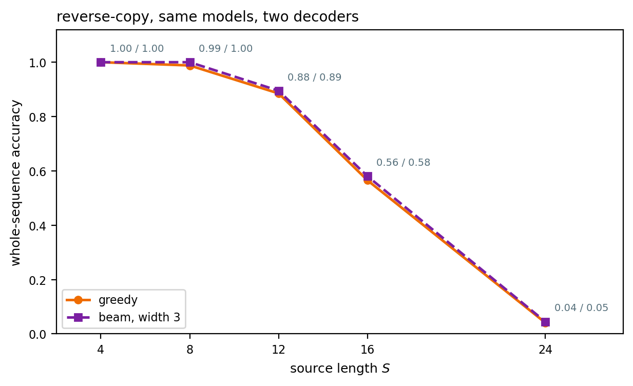
Measured

Same five trained models, decoded greedily and with a beam of 3
The beam adds at most one point of whole-sequence accuracy at any length, and none at \(S = 24\)

Cause

The search only reorders candidates by the model’s own scores
When the model’s factors are wrong because the summary lost the source, the best-scoring candidate is wrong too
On the published English-French system, widening the beam from 2 to 12 moved the ensemble from BLEU 33.0 to 34.5 (Sutskever et al. 2014)

Source of the loss

The per-step accuracy under teacher forcing fell with length on the same models: the summary, not the search

Training the Pair

Batches of Pairs Are Padded on Both Sides

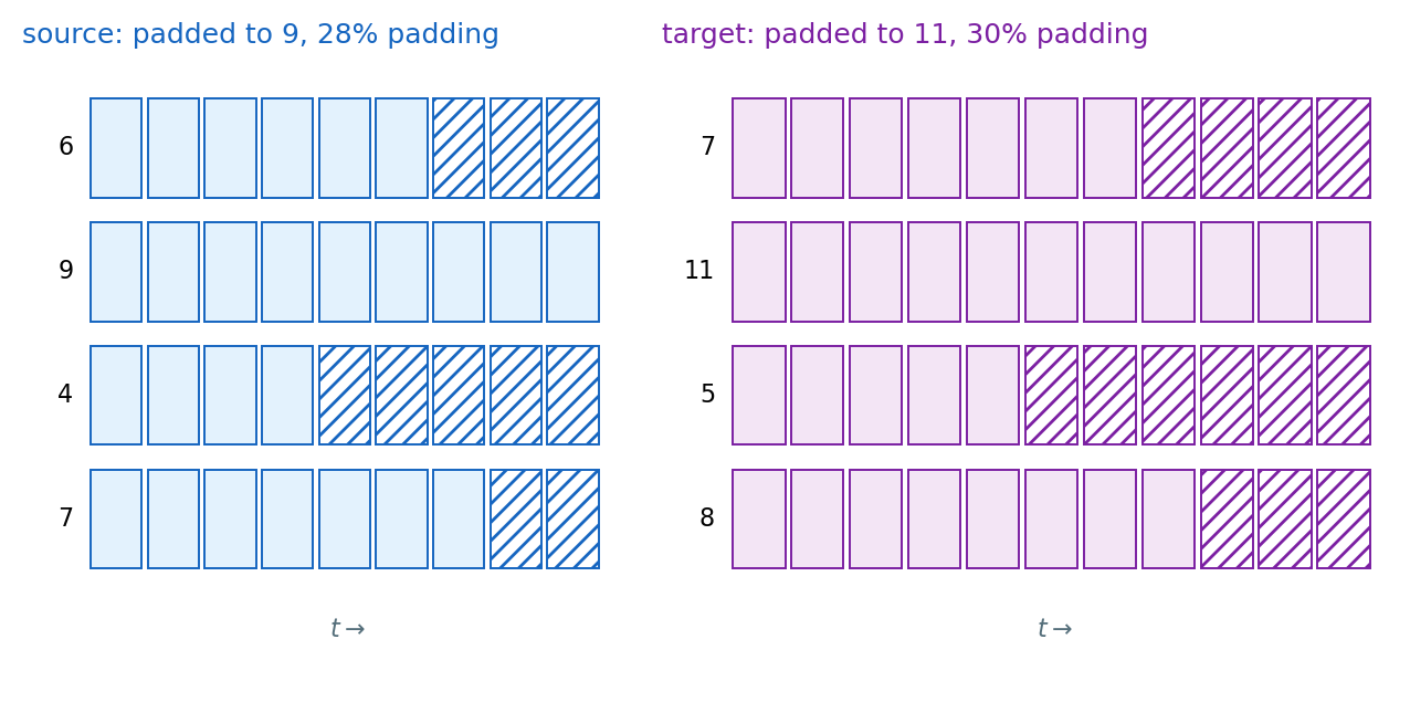
Two ragged sides

Each pair has its own source length \(S_n\) and target length \(T_n\)
A batch is two tensors, \((B, S_{\max})\) and \((B, T_{\max})\), each padded to its longest member with <pad>

Cost of the padding

Every pad cell is a full step of the reader or the writer, computed and discarded
The waste is \(1 - \sum_n S_n / (B \cdot S_{\max})\) on each side, and grows with the spread of lengths in the batch

Sorting by length

Group pairs of similar length into the same batch, so \(S_{\max}\) is close to every \(S_n\)
Batches are then drawn from length buckets, in random order across buckets
The published system sorted within windows of pairs so that a minibatch held sentences of about the same length

Masks Keep Padding Out of the Loss and Out of the Summary

Target side: mask the loss

\[L = -\frac{1}{\sum_{n,t} m_{n,t}} \sum_{n}\sum_{t=1}^{T_{\max}} m_{n,t}\, \log p(y_{n,t} \mid y_{n,<t}, \mathbf{x}_n), \qquad m_{n,t} = [t \le T_n]\]

Pad positions contribute nothing, and the average is over real words, not over cells
Without the mask the writer is trained to emit <pad> after <eos>, and the loss of a short pair is diluted by its padding

Source side: take the summary at the right step

The reader runs to \(S_{\max}\), but example \(n\)’s summary is its state at step \(S_n\), not at \(S_{\max}\)
After \(S_n\) the state has consumed pad embeddings and is no longer the summary of the sentence

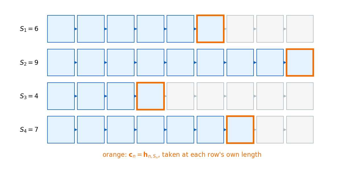
State carry-over, the general form

\[\mathbf{h}_{n,t} = m_{n,t}\, f(\mathbf{h}_{n,t-1}, \mathbf{x}_{n,t}) + (1 - m_{n,t})\, \mathbf{h}_{n,t-1}\]

A masked step leaves the state as it was, so the state at \(S_{\max}\) is the summary for every row

Packed Sequences Run the Reader on Real Steps Only

lengths = torch.tensor([6, 9, 4, 7])
packed = pack_padded_sequence(emb(src), lengths,
                              batch_first=True,
                              enforce_sorted=False)
out_packed, (h_n, c_n) = encoder(packed)
# h_n[-1][b] is row b's state at its own length

What packing does

Sorts the rows by length and stores, for each step \(t\), only the rows with \(S_n \ge t\)
Step \(t\) of the reader is one matrix product over the rows still active, so the batch shrinks as \(t\) grows
h_n holds each row’s state at its own last real step, and the mask on the state is no longer needed

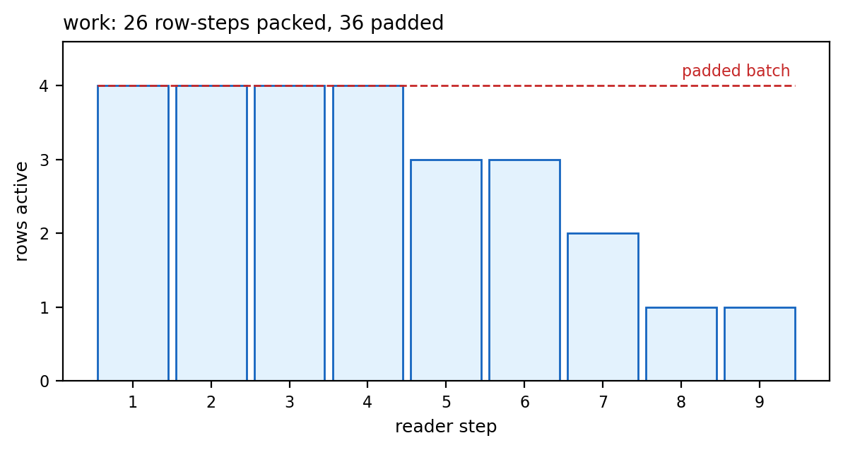
Cost

The work is \(\sum_n S_n\) row-steps instead of \(B \cdot S_{\max}\)
The per-step batch is smaller toward the end, so the last steps of the longest rows run at low hardware utilization

Published System Is Two Four-Layer LSTMs

	Value
Reader and writer	LSTM, 4 layers each, 1000 cells per layer
Embeddings	1000-dimensional, source and target
Vocabulary	160,000 source words, 80,000 target words, the rest mapped to `<unk>`
Parameters	384 million, of which 64 million are recurrent weights
Training data	12 million pairs, 348 million French words, 304 million English words
Source order	reversed
Optimization	SGD without momentum, learning rate 0.7, halved every half epoch after epoch 5, 7.5 epochs
Batches	128 pairs, sorted by length within windows
Gradient clipping	norm clipped at 5
Hardware and time	8 GPUs, one layer per GPU, about 10 days

Parameters

Two embedding tables and the readout hold 320 of the 384 million: \(160{,}000 \times 1000\), \(80{,}000 \times 1000\), and \(1000 \times 80{,}000\)
The eight recurrent layers hold the remaining 64 million

Time

The readout over 80,000 words at every target step
Four layers of recurrence, sequential in \(t\) on each side, for sentences of up to 80 words

Reversal, Ensembling, and a Wider Beam Were the Published Gains

System, WMT’14 English to French	BLEU
Single LSTM, source in order, beam 12	26.2
Single LSTM, source reversed, beam 12	30.6
Ensemble of 5 reversed LSTMs, beam 2	33.0
Ensemble of 5 reversed LSTMs, beam 12	34.8
Phrase-based baseline of the task	33.3
Best published WMT’14 result that year	37.0

Sutskever et al. 2014, Table 1 and Table 2, newstest2014

Row by row

Reversing the source: \(+4.4\) on a single model, the largest single change, with no new parameters
Five models trained from different initializations, their output distributions averaged at every step: \(+2.4\) at beam 2
A beam of 12 over a beam of 2: \(+1.8\)

Against the baselines

The first end-to-end neural system to pass the phrase-based baseline on this task, by 1.5 BLEU
Below the best system of the year, which combined phrase-based translation with neural rescoring

Metric

BLEU: overlap of the output’s word n-grams with reference translations, 0 to 100, with a penalty for short outputs

The Summary Is the Limit

Accuracy Falls with Source Length on One Trained Model

Measured

Per-step accuracy with every input given: 1.00 at \(S = 4\), 0.97 at \(S = 16\), 0.88 at \(S = 24\)
The whole sequence, feeding itself: 1.00, 0.57, 0.04

Published

On English-French with a fixed summary, BLEU falls with source length past about 20 words, while a system that reads every source position holds (Cho et al. 2014 and Bahdanau et al. 2015)
The published system’s reversal and ensembling raised the level and left the slope

Same model, longer input

Nothing in the model changes between \(S = 4\) and \(S = 24\): the same reader, the same writer, the same 128 numbers between them

Fixed Summaries Lose Information as the Source Grows

Demands on the summary

Hold every content word of the source and their order, in \(H\) numbers, for however many words there are
Be written by the reader one word at a time, so each word must survive every later word’s update
Be read by the writer one target word at a time, so each word must be retrievable from the same vector after any prefix

Two demands, on both sides

Retention: the first source word across \(S\) reader steps and \(T\) writer steps
Selectivity: the words in between must not overwrite it
A gated unit makes both trainable and neither unlimited

Remedies

Reversal: which source words are nearest the writer, not how many fit
A bidirectional reader: both ends of the source one step from the summary, the middle no nearer
Ensembles and a wider beam: the level of the whole curve, not its slope
A larger \(H\): more numbers, and a reader and writer that still have to place every word in them and retrieve it

Limit

One vector of fixed size between a source of any length and a target of any length
The reader computed one state per source position and kept none of them

Summary Holds the Last Words Read Best

Per-word accuracy

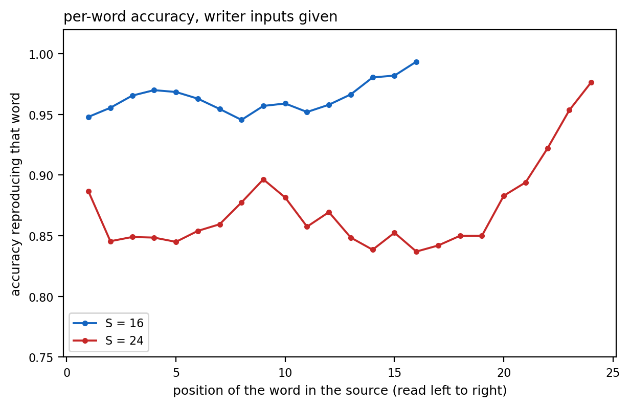
Same trained models, every writer input given, so each error is a word the summary did not deliver
Accuracy for each source word, by where that word sat in the source

Measured

\(S = 24\): the last three words read come back at 0.92 to 0.98, every earlier word at about 0.85
\(S = 16\): every word between 0.95 and 0.99, no clear plateau
The plateau does not fall with distance: the earliest word is reproduced as well as one in the middle

Capacity

The summary holds the most recent words at high accuracy and every earlier word at one shared, lower accuracy
More words share the same \(2H\) numbers as \(S\) grows, so the plateau drops
Every source word is present in the reader’s per-step states. Only the summary loses them

One Summary per Target Word

Each Target Word Needs Different Source Words

Per step

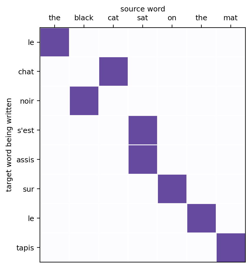
Writing “chat”: the source word “cat”. Writing “noir”: “black”, one position earlier in the source
Writing “s’est” and then “assis”: “sat” both times
A different source word, or a different pair of them, at almost every step

Fixed summary

The same vector \(\mathbf{c}\) at all eight steps, so every step has to extract its source word from one encoding of the whole sentence
The reader’s per-step states, \(\mathbf{h}_1, \ldots, \mathbf{h}_7\), each centred on one source word, are computed and not passed on

Open question

Whether the writer can be given, at each step, a vector built from the source words that step needs

Wider Summaries Hold the Source at Quadratic Cost

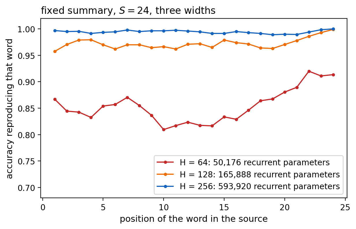
Measured at \(S = 24\)

\(H\)	Recurrent parameters	Mean per-word accuracy
64	50,176	0.854
128	165,888	0.972
256	593,920	0.994

Cost

Reader and writer each carry \(4(H^2 + H d)\) recurrent weights: doubling \(H\) roughly quadruples them
Every reader and writer step costs \(O(H^2)\), so the width is paid at every word of every sentence
The width that holds 24 words holds 24 words. A longer source needs a wider summary again

Unchanged by width

The source still reaches the writer as one vector, read in full at every target word
Which source word a target word draws on is still set inside that vector by the writer’s own recurrence

Writer Can Read Every Reader State with Weights from Content

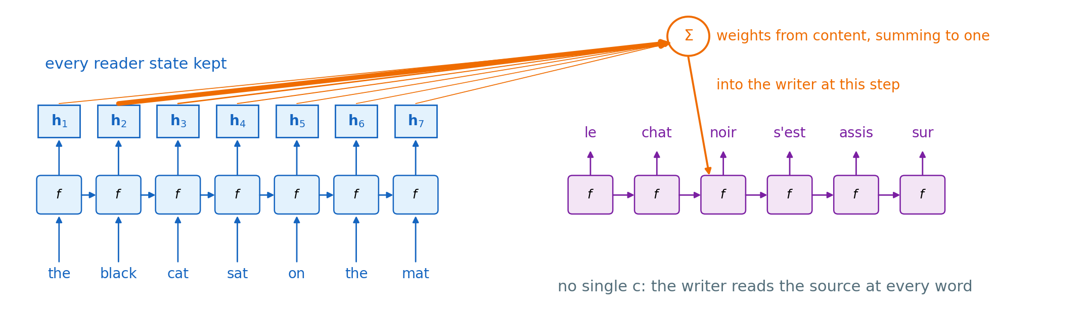
One summary per target word

\[\mathbf{c}_t = \sum_{s=1}^{S} a_{t,s}\,\mathbf{h}^{\text{enc}}_s, \qquad a_{t,s} = \frac{\exp(e_{t,s})}{\sum_{s'} \exp(e_{t,s'})}, \qquad e_{t,s} = \left(\mathbf{h}^{\text{dec}}_t\right)^{\!\top} \mathbf{h}^{\text{enc}}_s\]

Every reader state is kept: \(S\) vectors of \(H\) numbers
At each target word, one score per source position, from the writer’s state and that reader state, normalized to sum to one
\(\mathbf{c}_t\) is combined with the writer’s state before the readout

Added

No new recurrence: one dot product per source position and one weighted sum, at each target word
One matrix to combine \([\mathbf{h}^{\text{dec}}_t;\ \mathbf{c}_t]\), \(2H \times H\) parameters
The weights are not given: they are computed from the states, and the states are trained by the translation loss alone

Trained on the Same Task, Read Weights Place Each Output on Its Source Word

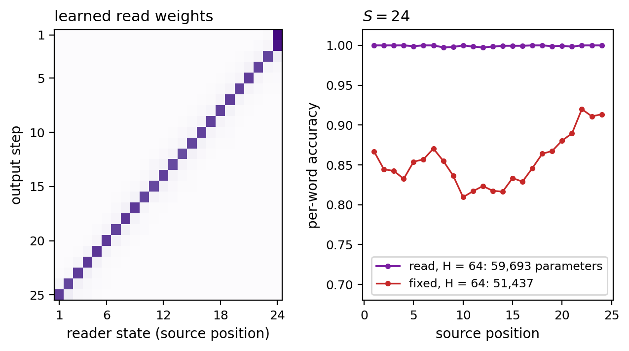
Measured at \(S = 24\), \(H = 64\)

Every source word reproduced at 0.998 or better, against 0.854 for the fixed summary of the same width
59,693 parameters in all, 16% more than the fixed-summary model
The fixed summary needed \(H = 256\) and twelve times the recurrent parameters to reach 0.994

Learned weights

Reverse-copy puts the last source word first, so the correct alignment is the reversed diagonal
Each output puts 0.78 to 0.98 of its weight on a single reader state, one step after the word it reproduces: the state whose most recent input is that word
No alignment was supplied. The weights were fitted by the same per-word cross-entropy as everything else

Gradient Reaches Each Source Word Through One Weighted Read

Two paths from a target word back to the source

\[\frac{\partial L_t}{\partial \mathbf{h}^{\text{enc}}_s} = \underbrace{a_{t,s}\,\frac{\partial L_t}{\partial \mathbf{c}_t}}_{\text{through the read}} + \ \underbrace{\frac{\partial L_t}{\partial \mathbf{h}^{\text{enc}}_S}\,\frac{\partial \mathbf{h}^{\text{enc}}_S}{\partial \mathbf{h}^{\text{enc}}_s}}_{\text{through the recurrence}} \;+\; \ldots\]

Through the read: one factor, the weight \(a_{t,s}\), at any distance between \(s\) and \(t\)
Through the recurrence: the product of reader Jacobians from step \(s\) to \(S\), then the writer’s steps, as with the fixed summary
Where the weight is large, the first path carries the gradient regardless of the source length

Training the weights

\(a_{t,s}\) depends on the states through the scores, so the gradient also adjusts where each target word reads
Backpropagation through the softmax and the dot products: no new training procedure

Cost per sentence pair

\(S \cdot T\) scores and \(T\) weighted sums of \(S\) vectors: \(O(S\,T\,H)\), against one read of \(\mathbf{c}\)
Memory: the \(S\) reader states, kept until the writer finishes, and an \(S \times T\) weight matrix for the backward pass

Unchanged

The reader still computes \(\mathbf{h}^{\text{enc}}_1, \ldots, \mathbf{h}^{\text{enc}}_S\) in sequence, and the writer its states in sequence
Each reader state is still the output of a recurrence: the read selects among states, and the recurrence still determines what each state holds

Read over every position, everywhere

The read gives any target word a one-step path to any source position
The same read applied among the positions of one sequence would give every position a one-step path to every other, at \(T^2\) scores per sequence and with no recurrence between them