Transformers and Self-Attention
EE 641 - Unit 6
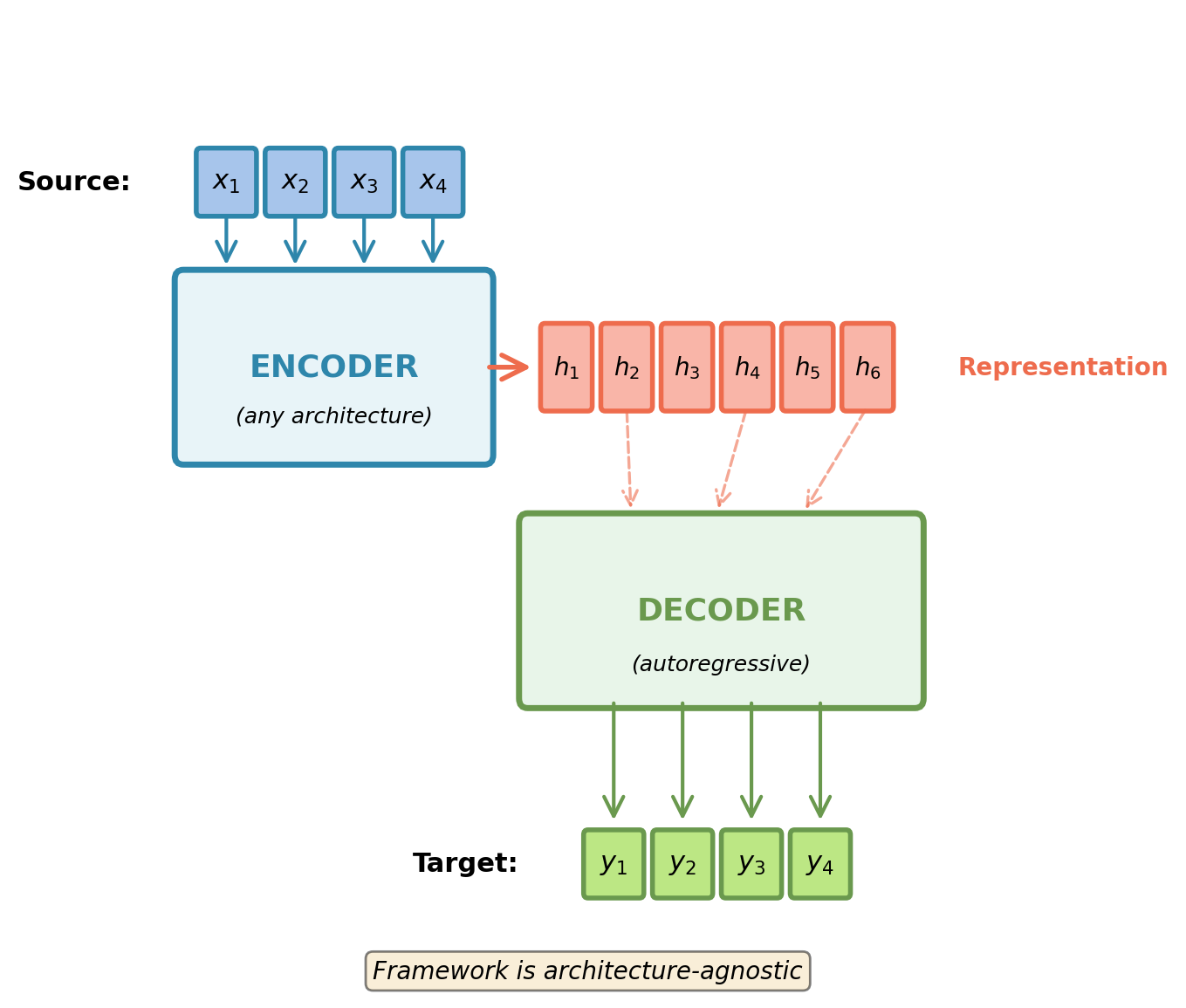
Information Flow: Understanding vs Generation
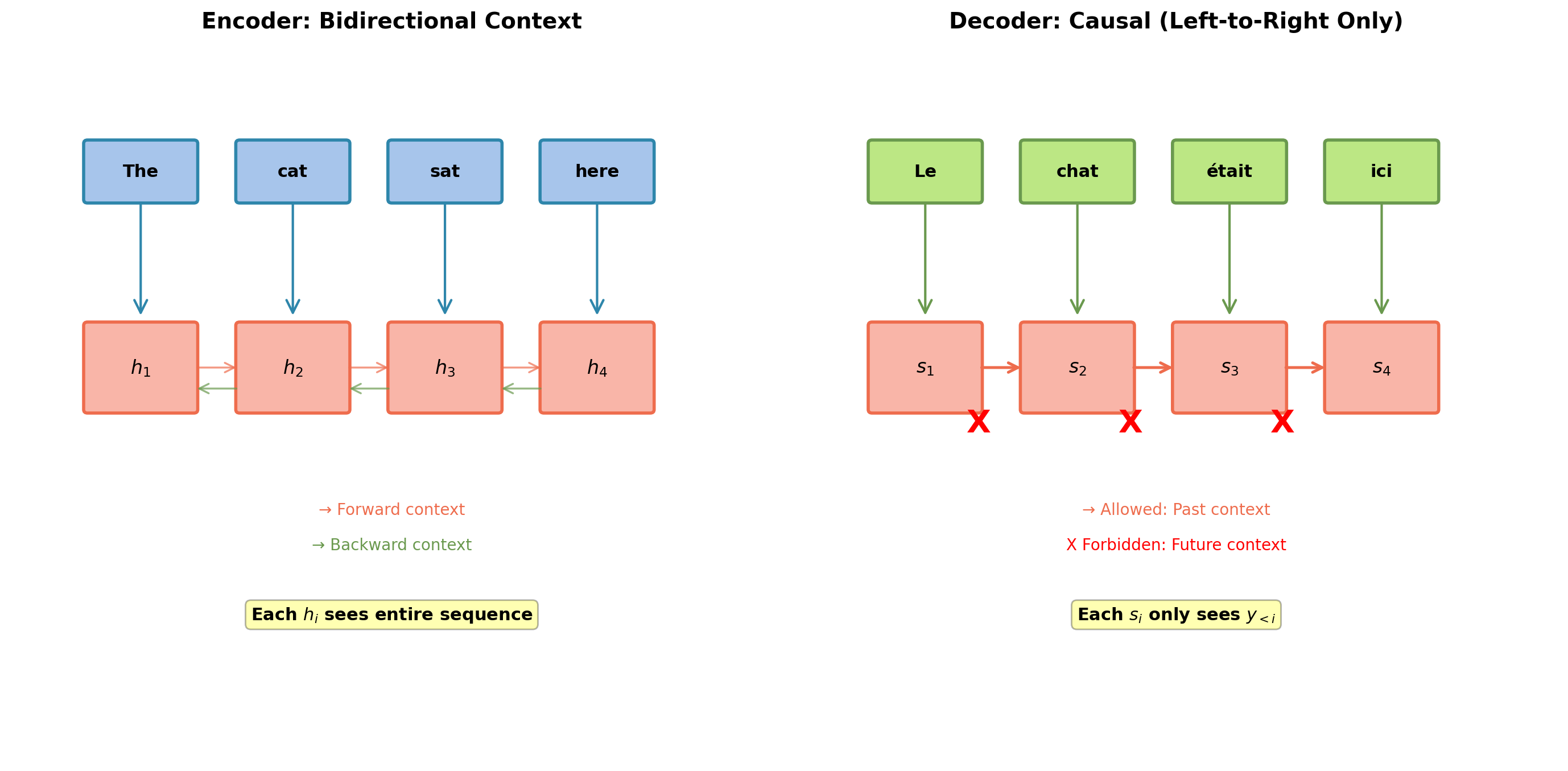
Encoder: Bidirectional context. Decoder: Causal constraint.
Cross-Attention: Connecting Encoder and Decoder
From Lecture 05: Attention Mechanism
Decoder queries encoder states: \[\mathbf{c}_t = \sum_{j=1}^{T_s} \alpha_{tj} \mathbf{h}_j\]
Where attention weights: \[\alpha_{tj} = \frac{\exp(e_{tj})}{\sum_{k=1}^{T_s} \exp(e_{tk})}\]
This is cross-attention:
- Query: Decoder state \(\mathbf{s}_{t-1}\)
- Keys/Values: Encoder states \(\{\mathbf{h}_j\}\)
- Dynamic selection of source information
Encoder representations are computed once and cached for all decoder timesteps.
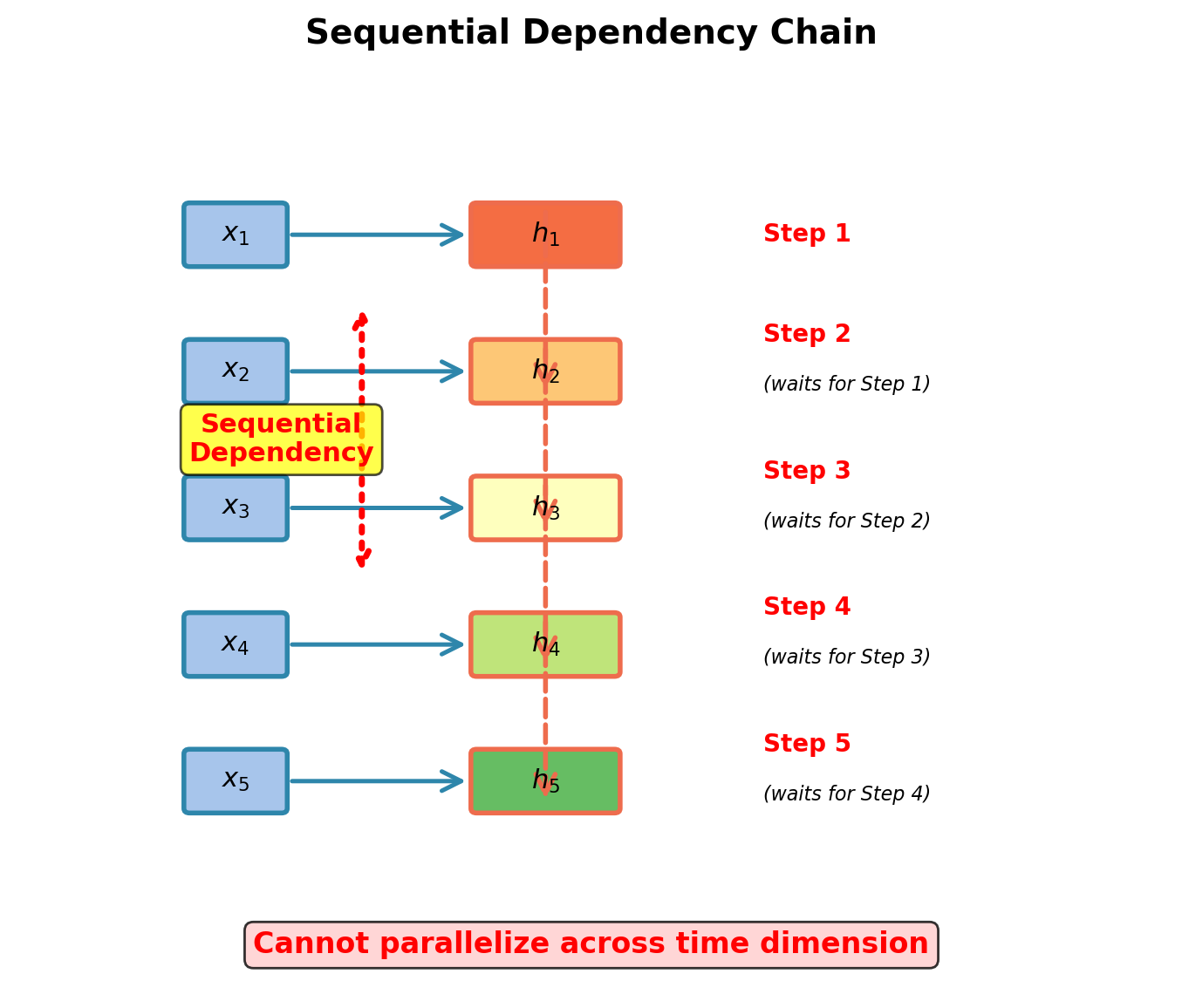
RNN Recurrence: Inherent Sequential Dependency
Fundamental constraint:
\[\mathbf{h}_t = f(\mathbf{x}_t, \mathbf{h}_{t-1})\]
Fundamental limitation:
- Must compute \(\mathbf{h}_1\) before \(\mathbf{h}_2\)
- Must compute \(\mathbf{h}_2\) before \(\mathbf{h}_3\)
- Cannot start \(\mathbf{h}_{10}\) until \(\mathbf{h}_9\) completes
Applies to encoding:
- Encoder has access to full source sequence
- Must still process sequentially
- 100-token sequence requires 100 sequential steps
- Hardware parallelism unutilized
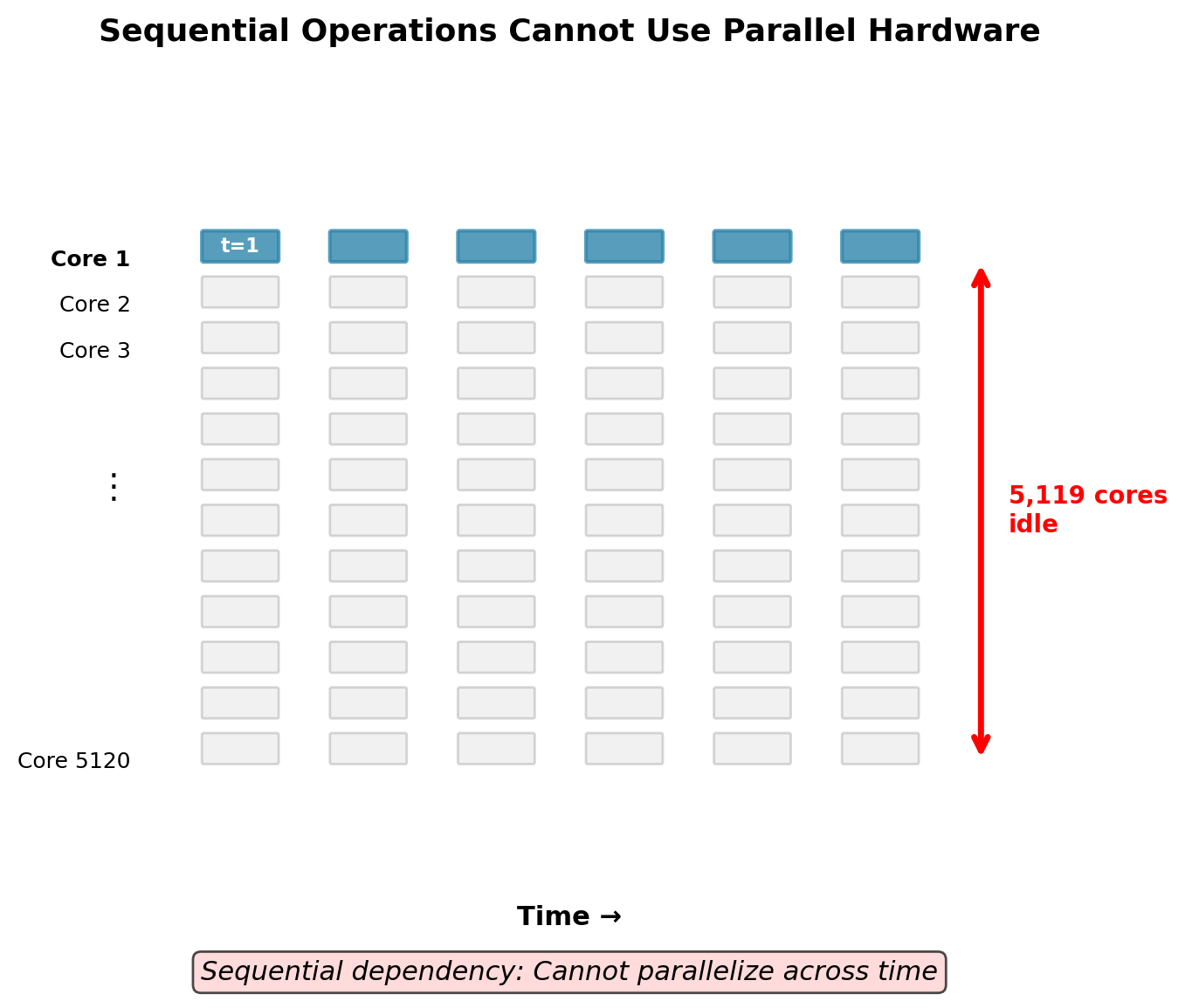
Hardware Utilization: RNNs Waste GPU Resources
RNN hidden state update rule:
\[\mathbf{h}_t = \tanh(\mathbf{W}_{hh}\mathbf{h}_{t-1} + \mathbf{W}_{xh}\mathbf{x}_t + \mathbf{b})\]
Where:
- \(\mathbf{h}_t, \mathbf{h}_{t-1} \in \mathbb{R}^d\) (hidden states)
- \(\mathbf{x}_t \in \mathbb{R}^{d_{in}}\) (input embedding)
- \(\mathbf{W}_{hh} \in \mathbb{R}^{d \times d}\) (recurrent weight matrix)
- \(\mathbf{W}_{xh} \in \mathbb{R}^{d \times d_{in}}\) (input weight matrix)
Critical observation:
- \(\mathbf{h}_{10}\) requires \(\mathbf{h}_9\)
- \(\mathbf{h}_9\) requires \(\mathbf{h}_8\)
- Cannot compute \(\mathbf{h}_{1:T}\) in parallel
GPU architecture mismatch:
- Modern GPU: 5,120 CUDA cores (V100)
- RNN forward pass: 1 active computation at a time
- Remaining 5,119 cores idle
- Utilization: Limited by Amdahl’s Law
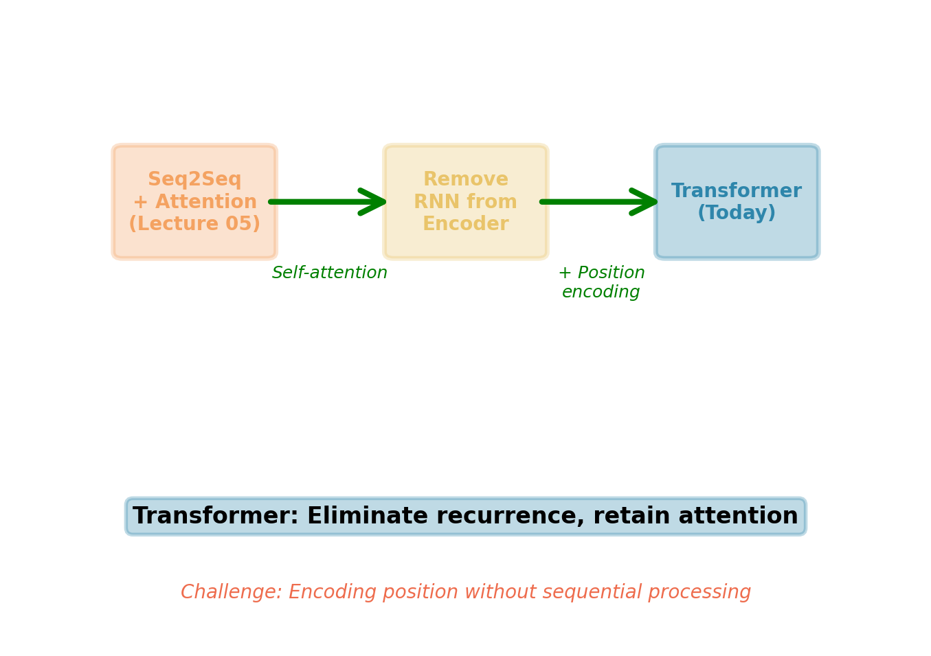
From Cross-Attention to Self-Attention
Attention mechanism achieve:
- Solved context bottleneck (variable-length representation)
- Provided direct gradient paths (no vanishing gradients over distance)
- Enabled content-based selection (dynamic alignment)
Remaining limitations:
- Encoder still uses RNN (sequential bottleneck for parallelization)
- RNN encoding still has vanishing gradients over long sequences
- Eliminating recurrence from encoding requires new approach
Transformer components:
Self-attention for encoding
- Every position attends to all positions
- Fully parallel computation
- Global receptive field from first layer
Positional encoding
- Attention is permutation-invariant
- Language is not: “dog bites man” ≠ “man bites dog”
- Explicit position injection breaks symmetry
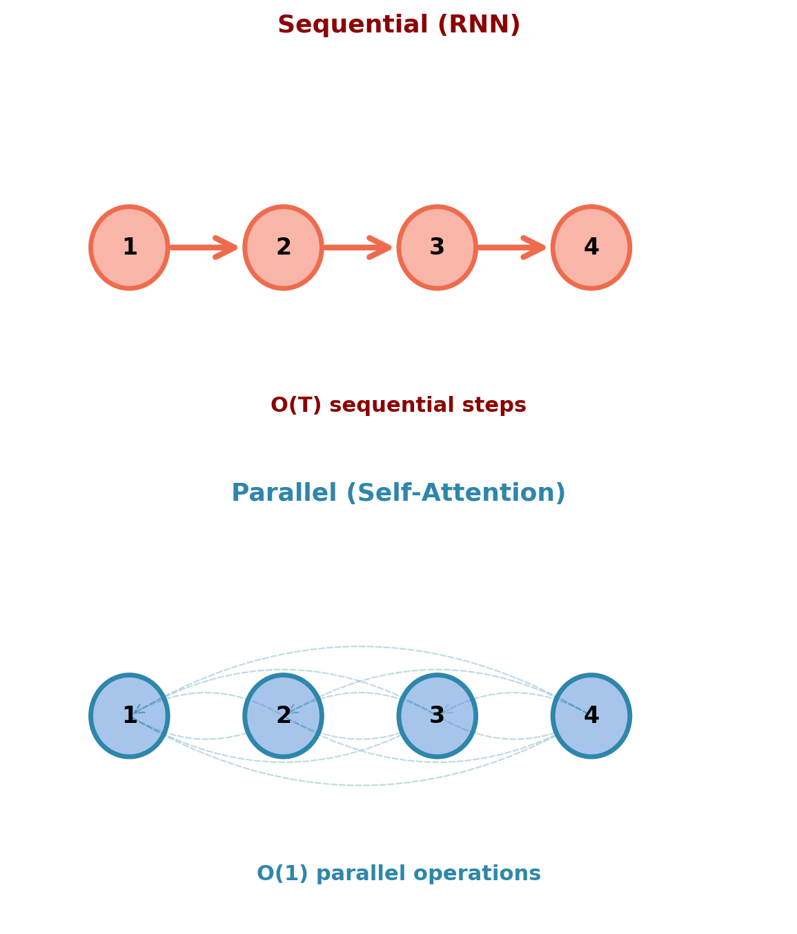
Rethinking Sequence Processing
Traditional view:
- Sequences processed sequentially: \(\mathbf{h}_t = f(\mathbf{x}_t, \mathbf{h}_{t-1})\)
- Each position depends on previous position
- Inherently serial computation
Alternative approach:
- Each position attends to all other positions simultaneously
- Replace sequential dependency with parallel all-to-all connections
- No recurrence needed if direct access exists everywhere
What changes:
- Instead of: “Position \(t\) waits for position \(t-1\)”
- Now: “Position \(t\) sees all positions at once”
- Computation becomes: \(\mathbf{h}_t = g(\mathbf{x}_t, \{\mathbf{x}_j\}_{j=1}^T)\) for all \(t\) in parallel
Self-Attention: Every Position Attends to Every Position
Cross-attention:
- Decoder attends to encoder states
- Query: From decoder \(\mathbf{s}_{t-1}\)
- Keys/Values: From encoder \(\{\mathbf{h}_j\}\)
- Different sequences interact
Self-attention:
- Sequence attends to itself
- Query, Key, Value: All from same sequence
- Every position can see every other position
- Build contextual representations without recurrence
Mathematical form:
For input sequence \(\mathbf{X} = [\mathbf{x}_1, \ldots, \mathbf{x}_T] \in \mathbb{R}^{T \times d}\):
\[\mathbf{h}_t = \sum_{j=1}^T \alpha_{tj} \mathbf{x}_j\]
where \(\alpha_{tj}\) measures similarity between position \(t\) and position \(j\).
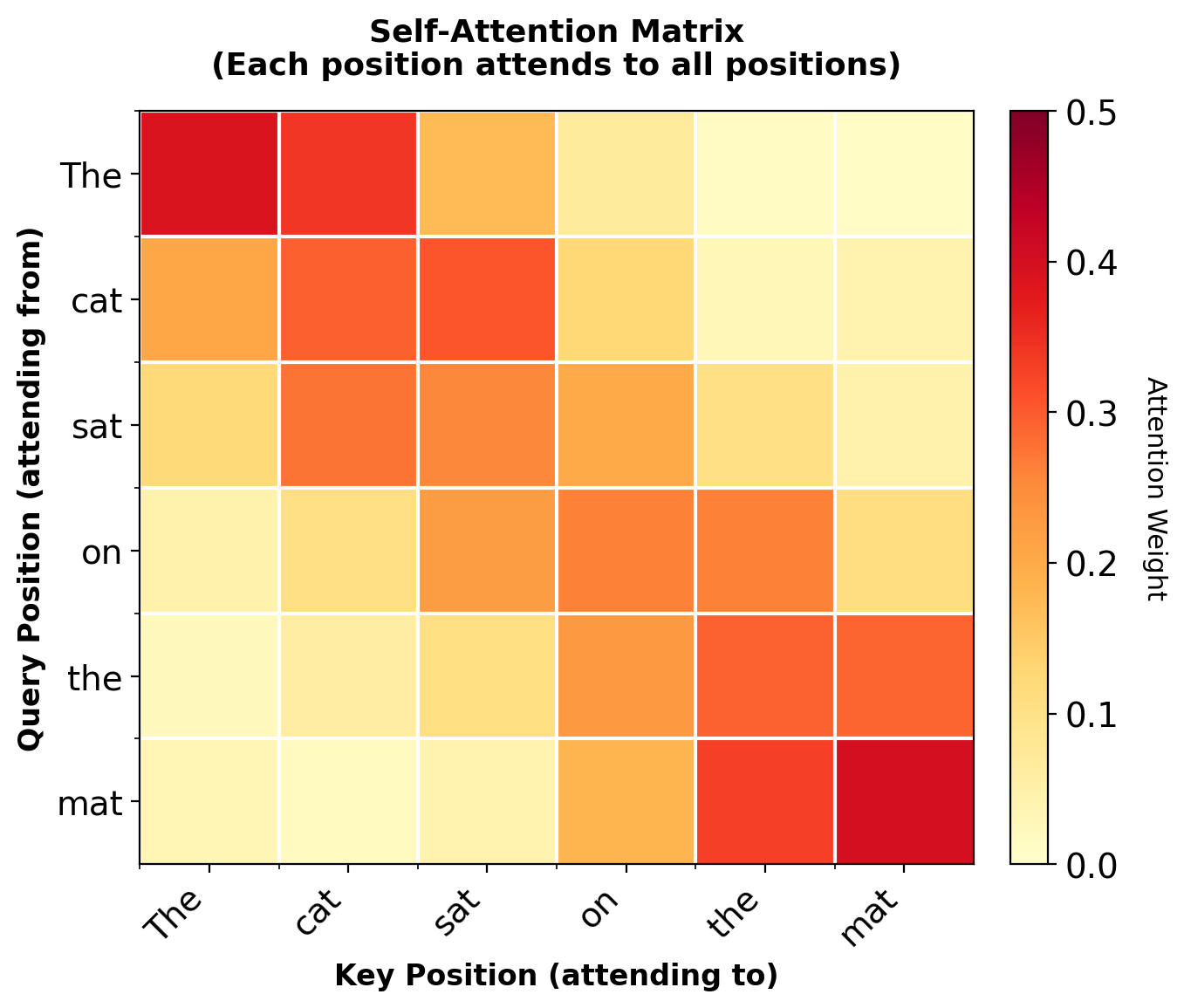
Diagonal elements (self-attention) are non-zero. Each position can attend to itself.
Parallelization: All Positions Computed Simultaneously
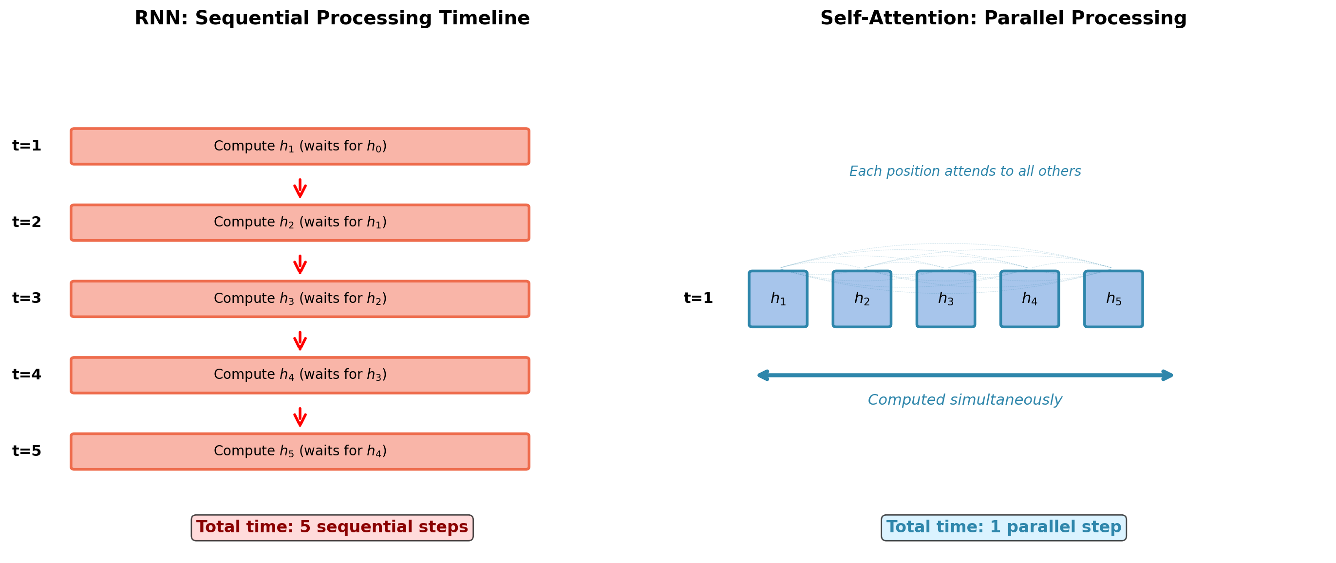
For \(T=100\) tokens, RNN requires 100 sequential operations. Self-attention: 1 parallel operation.
Computational Tradeoff: Memory for Speed
RNN complexity:
- Operations: \(O(T \times d^2)\) FLOPs
- Sequential depth: \(O(T)\) steps
- Memory: \(O(T \times d)\) for hidden states
- Cannot parallelize across time
For \(T=100\), \(d=512\):
- Total FLOPs: \(100 \times 512^2 = 26.2M\)
- Sequential steps: 100
- Memory: \(100 \times 512 = 51K\) values
Self-Attention complexity:
- Operations: \(O(T^2 \times d)\) FLOPs
- Sequential depth: \(O(1)\) steps
- Memory: \(O(T^2 + T \times d)\) for attention + representations
- Fully parallelizable
For \(T=100\), \(d=512\):
- Total FLOPs: \(100^2 \times 512 = 5.12M\)
- Sequential steps: 1
- Memory: \(100^2 + 100 \times 512 = 61K\) values
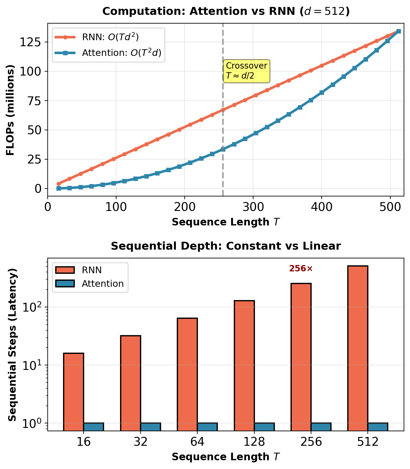
Attention has constant latency regardless of sequence length.
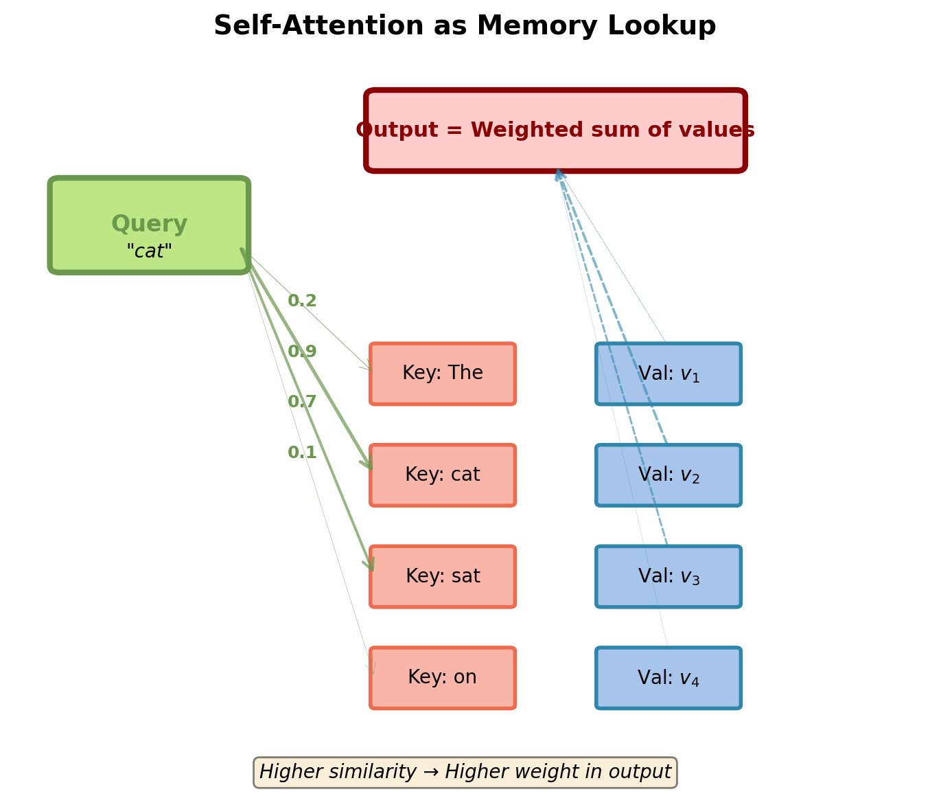
Database Analogy: Query, Key, Value
Attention as differentiable database lookup:
Database has:
- Keys: What to match against (identifier)
- Values: What to return (content)
Query:
- What to retrieve
- Compared against all keys
Retrieval:
- Find keys similar to query
- Return weighted average of corresponding values
In self-attention:
- Every position generates Q, K, and V
- Position acts as query to look up other positions
- Also provides key and value for other queries
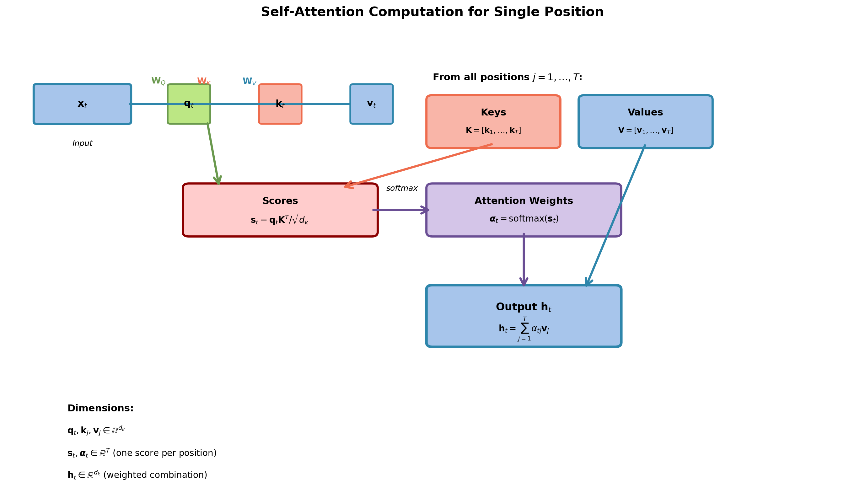
Mathematical Formulation of Self-Attention
Input sequence: \(\mathbf{X} = [\mathbf{x}_1, \ldots, \mathbf{x}_T] \in \mathbb{R}^{T \times d}\)
Linear projections:
\[\mathbf{Q} = \mathbf{X}\mathbf{W}_Q, \quad \mathbf{K} = \mathbf{X}\mathbf{W}_K, \quad \mathbf{V} = \mathbf{X}\mathbf{W}_V\]
Where \(\mathbf{W}_Q, \mathbf{W}_K, \mathbf{W}_V \in \mathbb{R}^{d \times d_k}\) are learned projection matrices, producing \(\mathbf{Q}, \mathbf{K}, \mathbf{V} \in \mathbb{R}^{T \times d_k}\).
Attention computation:
\[\text{Attention}(\mathbf{Q}, \mathbf{K}, \mathbf{V}) = \text{softmax}\left(\frac{\mathbf{QK}^T}{\sqrt{d_k}}\right)\mathbf{V}\]
Step by step:
- Compute similarity scores: \(\mathbf{S} = \mathbf{QK}^T \in \mathbb{R}^{T \times T}\)
- Scale: \(\mathbf{S} = \mathbf{S} / \sqrt{d_k}\)
- Normalize: \(\mathbf{A} = \text{softmax}(\mathbf{S}) \in \mathbb{R}^{T \times T}\)
- Weighted sum: \(\mathbf{H} = \mathbf{AV} \in \mathbb{R}^{T \times d_k}\)
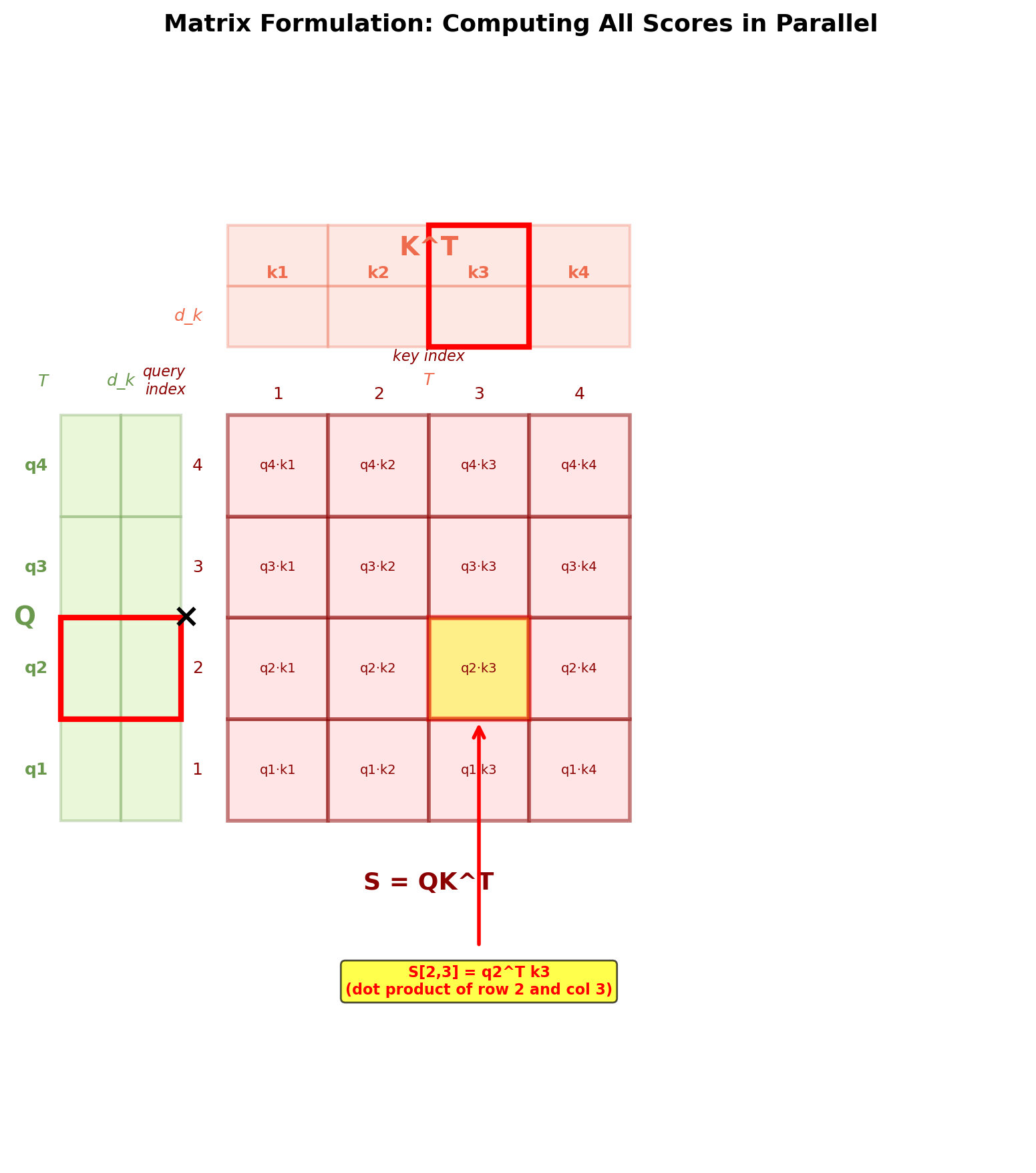
Each cell \(S[i,j] = q_i^T k_j\) is one dot product between query \(i\) and key \(j\). Matrix formulation enables parallel computation of all pairwise scores.
Sequential (nested loops):
T² sequential operations.
Parallel (matrix multiply):
All T² dot products computed simultaneously in one GPU kernel.
Why Separate Q, K, V Projections?
Without separation: \(\text{Attention}(\mathbf{X}, \mathbf{X}, \mathbf{X})\)
- Same representation for all three roles
- Symmetric similarity: \(\text{sim}(\mathbf{x}_i, \mathbf{x}_j) = \text{sim}(\mathbf{x}_j, \mathbf{x}_i)\)
- Limited expressiveness
With separation: Separate projection matrices
- Query space: “What am I looking for?”
- Key space: “What identifying features do I expose?”
- Value space: “What information do I provide when selected?”
Allows asymmetric relationships:
- “cat” (query) can strongly attend to “sat” (key)
- But “sat” (query) may weakly attend to “cat” (key)
- Learned from data, not enforced by architecture
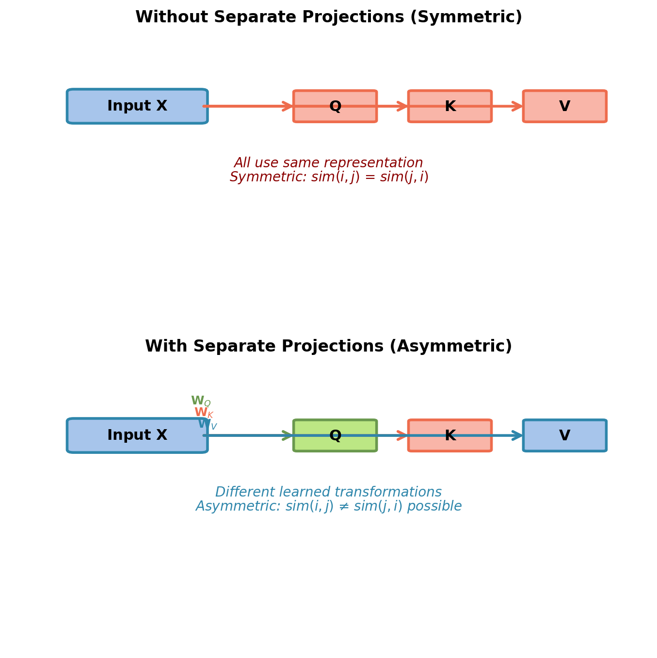
Example: “subject” query can match “verb” keys strongly, while “verb” query matches “object” keys.
Self-Attention Computation Flow
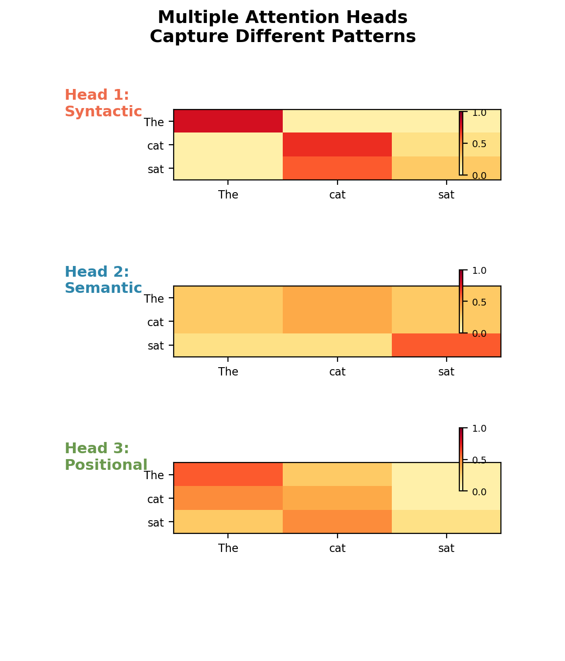
Motivation: Multiple Types of Relationships
Single attention captures one similarity function.
Language has multiple simultaneous relationships:
- Syntactic: Subject-verb agreement, modifier-noun
- Semantic: Synonyms, antonyms, related concepts
- Positional: Previous token, next token, fixed offsets
- Discourse: Coreference, anaphora resolution
Solution: Multiple attention heads
- Run multiple attention operations in parallel
- Each head can learn different relationship types
- Heads operate independently
- Combine outputs at the end
Analogy: Multiple convolutional filters in CNN, each detecting different features.
Each head specializes in different attention patterns.
Multi-Head Attention: Mathematical Formulation
Divide model dimension into \(h\) heads:
\[d_{model} = h \times d_k\]
For each head \(i \in \{1, \ldots, h\}\):
\[\text{head}_i = \text{Attention}(\mathbf{X}\mathbf{W}_i^Q, \mathbf{X}\mathbf{W}_i^K, \mathbf{X}\mathbf{W}_i^V)\]
Where:
- \(\mathbf{W}_i^Q, \mathbf{W}_i^K \in \mathbb{R}^{d_{model} \times d_k}\)
- \(\mathbf{W}_i^V \in \mathbb{R}^{d_{model} \times d_v}\)
- Typically \(d_k = d_v = d_{model}/h\)
Concatenate and project:
\[\text{MultiHead}(\mathbf{X}) = \text{Concat}(\text{head}_1, \ldots, \text{head}_h)\mathbf{W}^O\]
Where \(\mathbf{W}^O \in \mathbb{R}^{h \cdot d_v \times d_{model}}\)
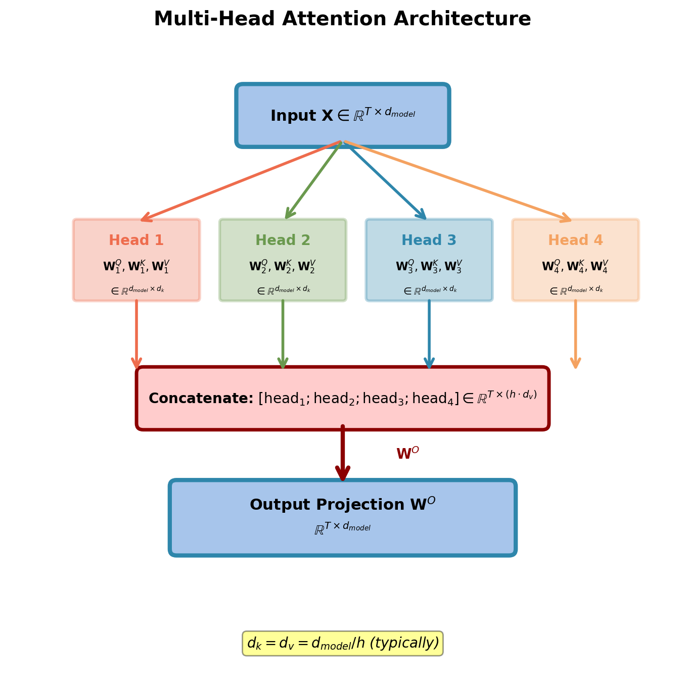
Total parameters: Same as single attention head at full dimension.
Computational Efficiency of Multi-Head Attention
Single-head attention at full dimension:
- Query, Key, Value: \(3 \times (d_{model} \times d_{model})\) parameters
- Attention computation: \(O(T^2 \times d_{model})\) FLOPs
Multi-head with \(h\) heads:
- Per head: \(3 \times (d_{model} \times d_k)\) where \(d_k = d_{model}/h\)
- Total: \(h \times 3 \times (d_{model} \times d_{model}/h) = 3 \times d_{model}^2\)
- Output projection: \(d_{model}^2\)
- Total attention: \(O(T^2 \times d_{model})\) FLOPs
Same total parameters and FLOPs.
But with benefits:
- Smaller matrices per head: Better GPU cache utilization
- Parallel computation: All heads computed simultaneously
- Multiple representation subspaces: Richer expressiveness
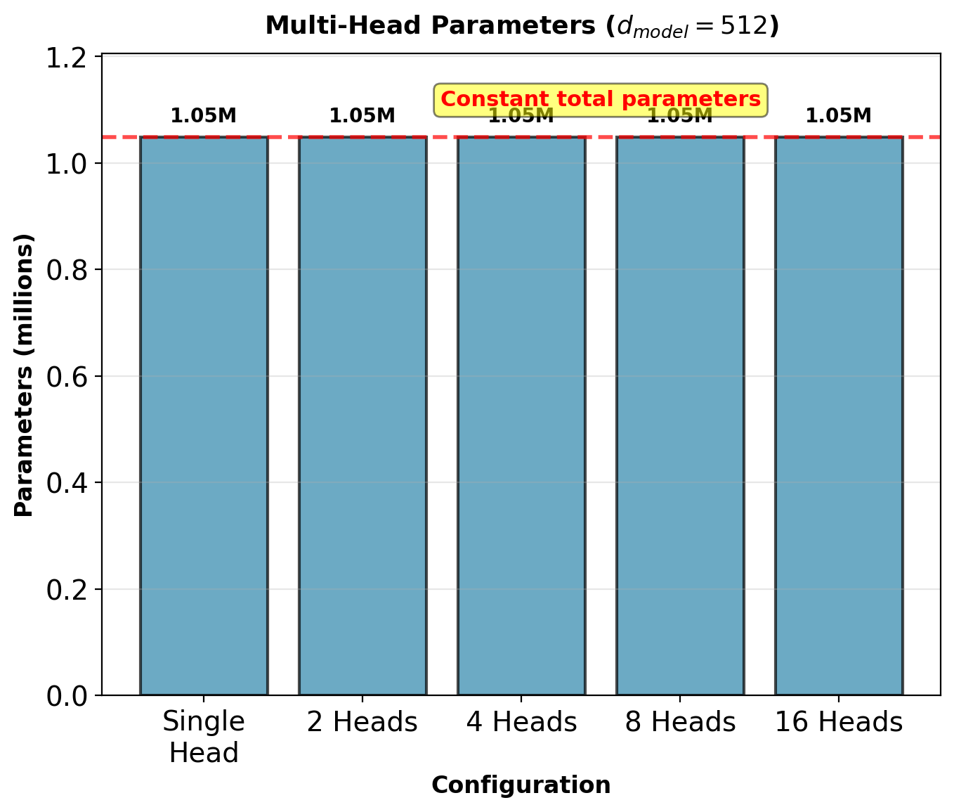
Dimension per head: \(d_k = d_{model}/h = 512/8 = 64\) (for 8 heads)
Smaller per-head dimension improves cache locality.
What Different Heads Learn: Empirical Analysis
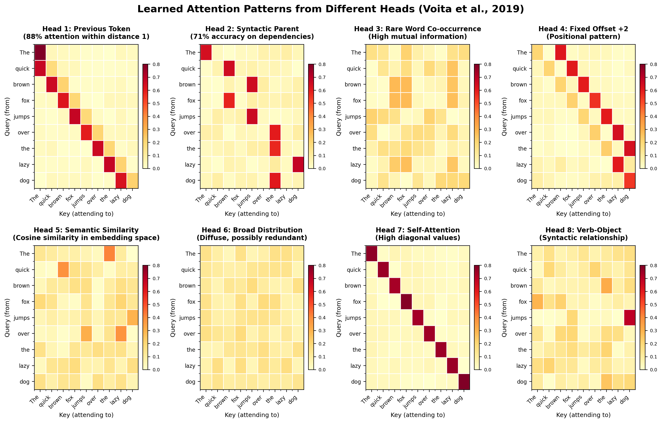
Different heads specialize without supervision. Patterns emerge from data.
Ablation Study: Impact of Number of Heads
WMT’14 En→De Translation (from “Attention Is All You Need”):
| Heads | \(d_k\) | BLEU | Training Time |
|---|---|---|---|
| 1 | 512 | 25.1 | 1.0× |
| 2 | 256 | 26.4 | 0.98× |
| 4 | 128 | 27.1 | 1.02× |
| 8 | 64 | 27.3 | 1.0× |
| 16 | 32 | 26.9 | 1.05× |
| 32 | 16 | 25.8 | 1.12× |
Observations:
- 1 head: -2.2 BLEU (significant degradation)
- 8 heads: Optimal for this task
- 16+ heads: Slight degradation (too many redundant heads)
- Too small \(d_k\) (<32): Insufficient capacity per head
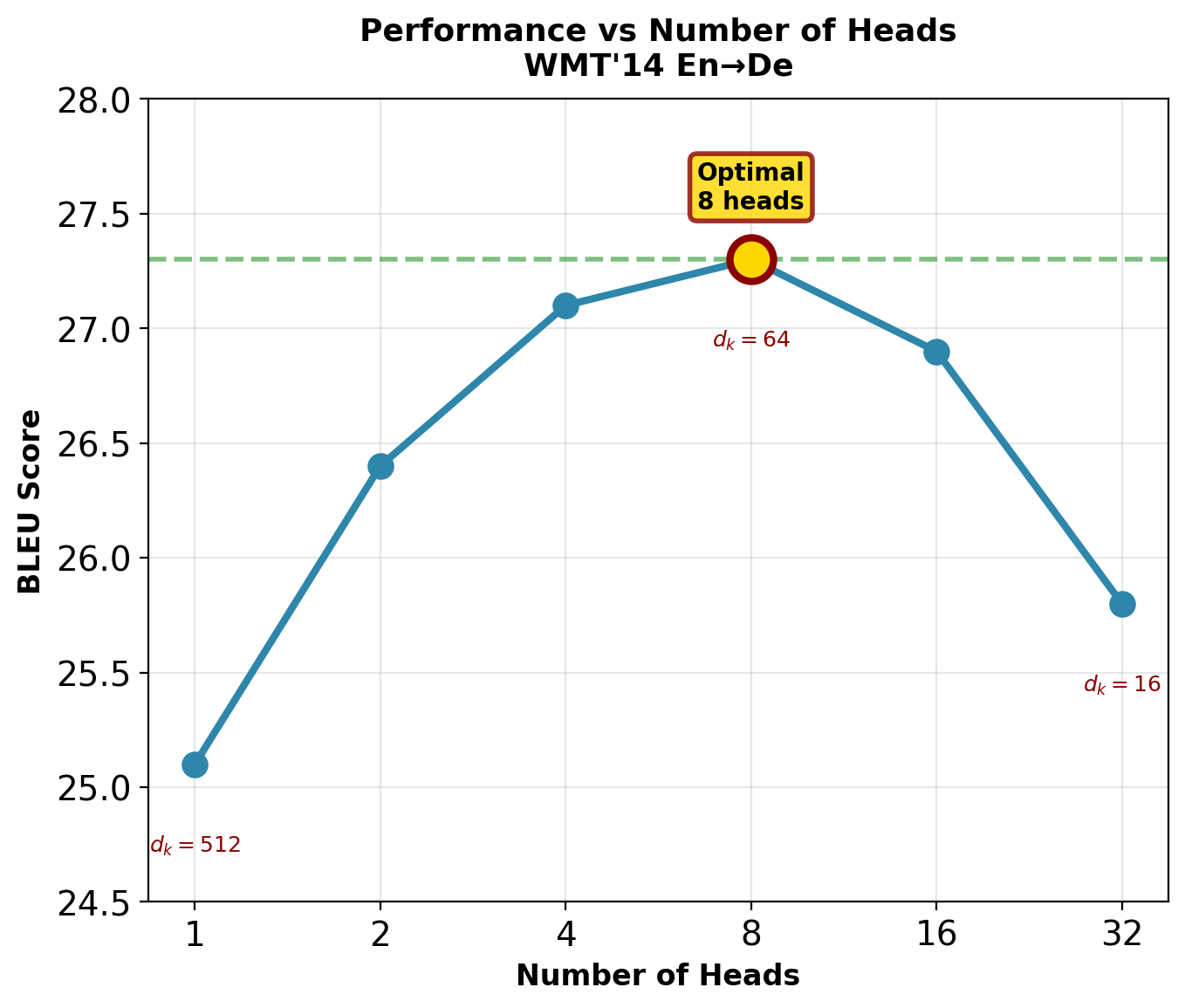
8 heads with \(d_k=64\) balances expressiveness and efficiency.
Head Pruning: Some Heads Are Redundant
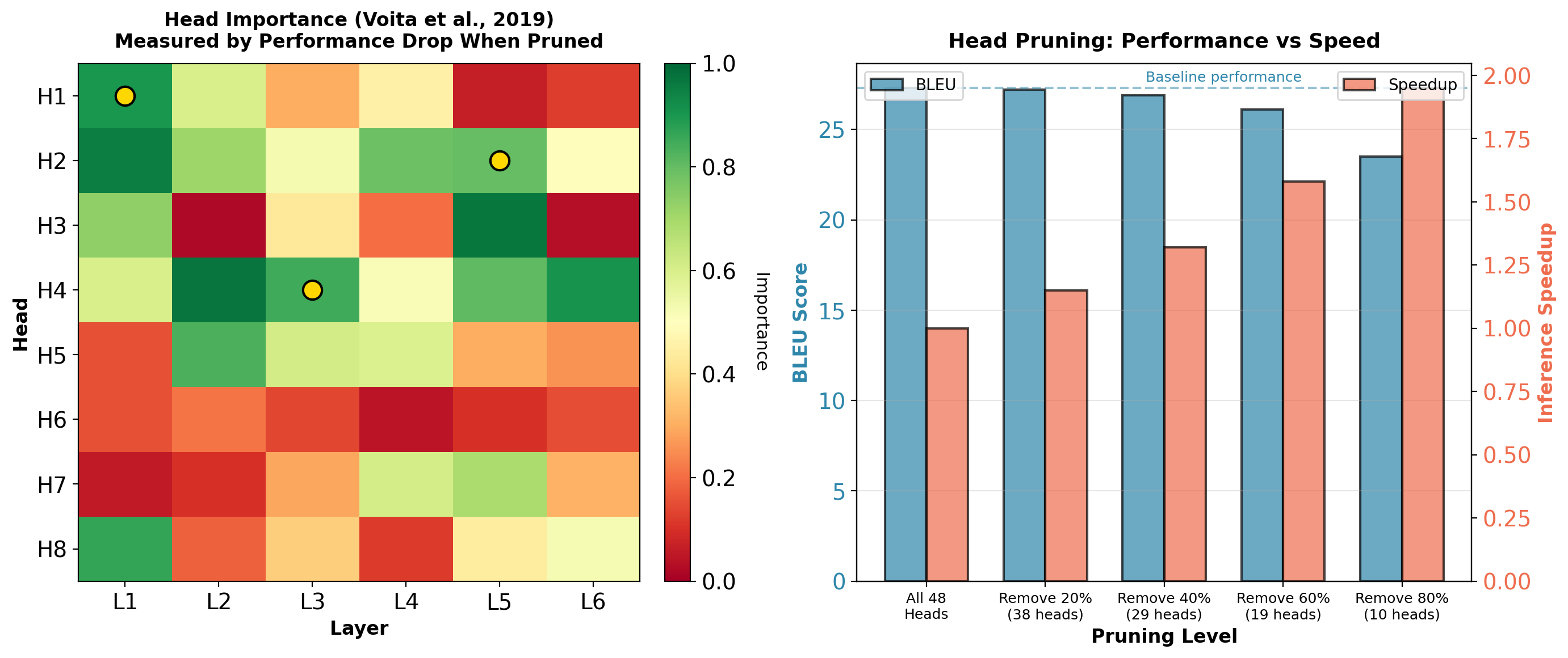
Can remove 40% of heads with <0.5 BLEU loss and 1.3× speedup. Some heads are redundant or specialized for rare patterns.
Why Scaling Matters in Self-Attention
Recall: Scaled dot-product attention
\[\text{Attention}(\mathbf{Q}, \mathbf{K}, \mathbf{V}) = \text{softmax}\left(\frac{\mathbf{QK}^T}{\sqrt{d_k}}\right)\mathbf{V}\]
Why divide by \(\sqrt{d_k}\)?
In self-attention, all \(T\) positions compete for attention weight. Without scaling:
- Dot products \(\mathbf{q}_i \cdot \mathbf{k}_j\) grow with dimension \(d_k\)
- For large \(d_k\), scores become very large
- Softmax saturates: One position gets ~1.0, others get ~0
- Gradients vanish for non-dominant positions
Problem amplified in self-attention:
- Every position must attend somewhere (weights sum to 1)
- With \(T\) positions, need stable gradients for all
- Saturation prevents learning diverse attention patterns
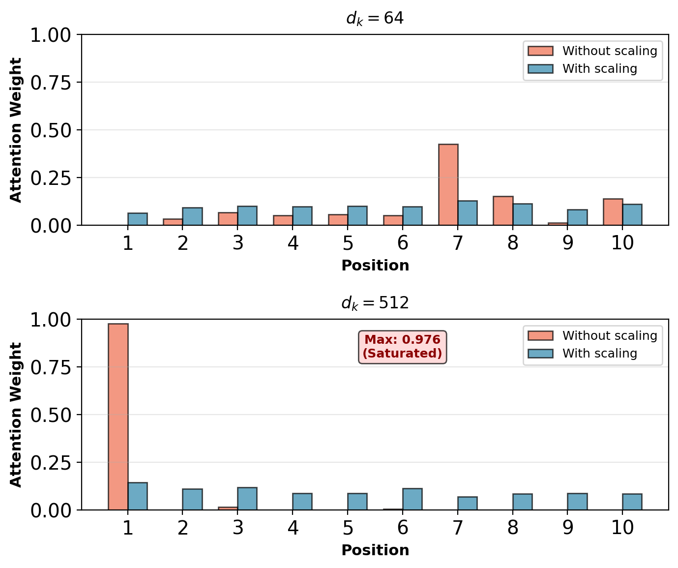
Without scaling, large \(d_k\) causes attention saturation.
Variance Analysis: Why \(\sqrt{d_k}\)?
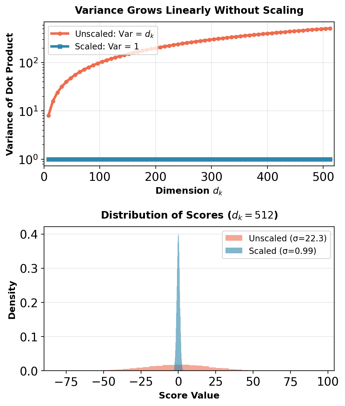
Assume query and key components are independent with unit variance:
\[\mathbf{q}, \mathbf{k} \sim \mathcal{N}(0, \mathbf{I})\]
Dot product without scaling:
\[\mathbf{q} \cdot \mathbf{k} = \sum_{i=1}^{d_k} q_i k_i\]
Each term \(q_i k_i\) has:
- \(\mathbb{E}[q_i k_i] = \mathbb{E}[q_i]\mathbb{E}[k_i] = 0 \times 0 = 0\)
- \(\text{Var}(q_i k_i) = \mathbb{E}[q_i^2 k_i^2] = \mathbb{E}[q_i^2]\mathbb{E}[k_i^2] = 1 \times 1 = 1\)
Sum of \(d_k\) independent random variables:
\[\text{Var}(\mathbf{q} \cdot \mathbf{k}) = \sum_{i=1}^{d_k} \text{Var}(q_i k_i) = d_k\]
After scaling by \(1/\sqrt{d_k}\):
\[\text{Var}\left(\frac{\mathbf{q} \cdot \mathbf{k}}{\sqrt{d_k}}\right) = \frac{1}{d_k} \text{Var}(\mathbf{q} \cdot \mathbf{k}) = \frac{d_k}{d_k} = 1\]
Variance is stabilized regardless of dimension.
Attention Entropy: Measuring Distribution Sharpness
Entropy of attention distribution:
\[H(\boldsymbol{\alpha}_t) = -\sum_{j=1}^T \alpha_{tj} \log \alpha_{tj}\]
Interpretation:
- \(H = 0\): Attention fully concentrated on one position
- \(H = \log T\): Uniform distribution (maximum entropy)
- Higher entropy: More diverse attention
Without scaling:
- Large \(d_k\) causes low entropy (peaked distribution)
- Model forced to focus on single position
- Cannot learn soft combinations
With scaling:
- Entropy controlled by learned scores, not dimension
- Model can choose concentration level
- Enables both sharp and soft attention
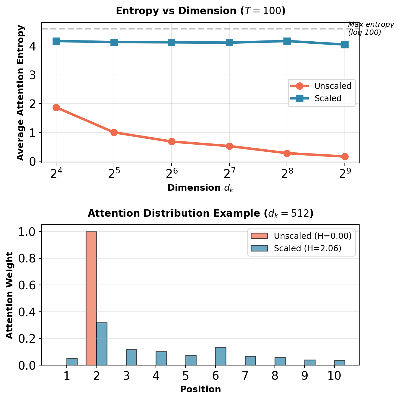
Scaling preserves entropy across dimensions, enabling diverse attention patterns.
Temperature as Generalization of Scaling
Attention with temperature \(\tau\):
\[\text{Attention}(\mathbf{Q}, \mathbf{K}, \mathbf{V}, \tau) = \text{softmax}\left(\frac{\mathbf{QK}^T}{\tau}\right)\mathbf{V}\]
Standard scaling: \(\tau = \sqrt{d_k}\)
Temperature effects:
- \(\tau \to 0\): Approaches hard attention (argmax)
- \(\tau < \sqrt{d_k}\): Sharper distribution (more peaked)
- \(\tau = \sqrt{d_k}\): Standard scaling (stable training)
- \(\tau > \sqrt{d_k}\): Softer distribution (more uniform)
- \(\tau \to \infty\): Uniform attention (all positions equal weight)
Application: Can adjust temperature at inference for diversity.
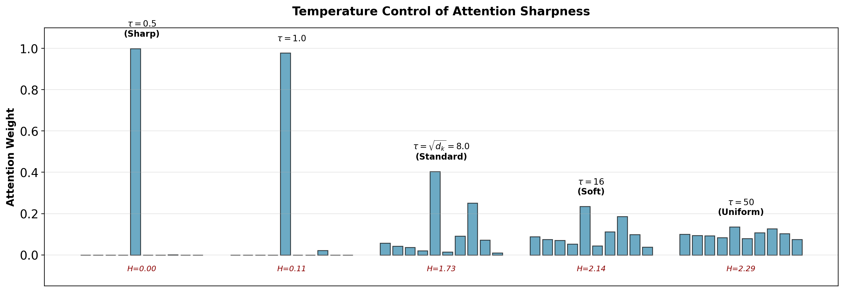
Temperature provides control over attention concentration. Standard \(\tau = \sqrt{d_k}\) balances sharpness and diversity.
Self-Attention is Permutation Invariant
Matrix operations preserve set structure, not sequence order.
Consider self-attention computation: \[\mathbf{h}_i = \sum_{j=1}^T \alpha_{ij} \mathbf{v}_j\]
where attention weights depend only on content: \[\alpha_{ij} = \text{softmax}(\mathbf{q}_i^T \mathbf{k}_j / \sqrt{d_k})\]
Key observation:
- If we permute input \(\mathbf{X} \to \mathbf{X}_\pi\)
- Query, key, value all permute: \(\mathbf{Q}_\pi, \mathbf{K}_\pi, \mathbf{V}_\pi\)
- Attention scores permute: \(\alpha_{ij}\) becomes \(\alpha_{\pi(i)\pi(j)}\)
- Output permutes identically: \(\mathbf{H} \to \mathbf{H}_\pi\)
Mathematical property: \[\text{SelfAttention}(\mathbf{X}_\pi) = \text{SelfAttention}(\mathbf{X})_\pi\]
Self-attention is permutation equivariant: Permute input → same permutation of output.
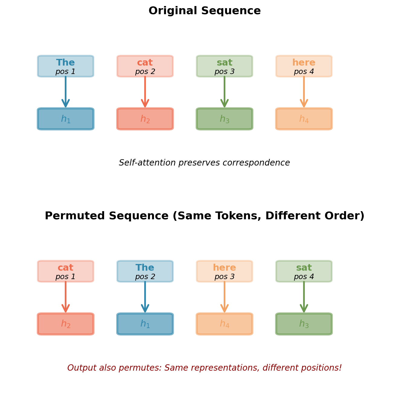
Each token gets same contextual representation regardless of where it appears.
Language is NOT Permutation Invariant
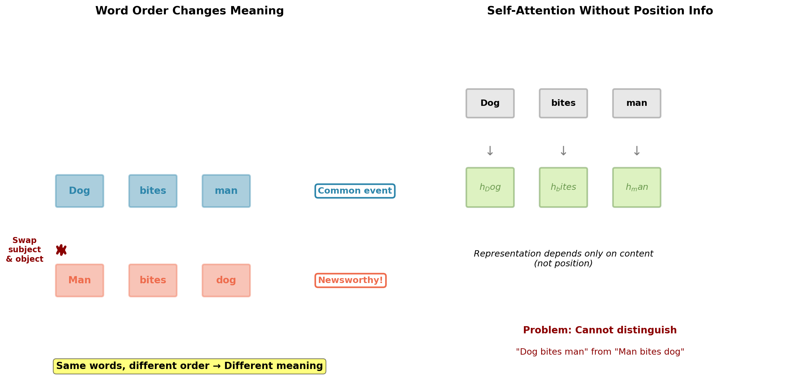
Critical limitation: Pure self-attention treats sequences as sets, not ordered sequences.
Requirements for Position Information
Position information requires vectors \(\mathbf{p}_t \in \mathbb{R}^{d_{model}}\) that satisfy:
Requirement 1: Uniqueness
Each position must have distinct encoding: \[\mathbf{p}_i \neq \mathbf{p}_j \text{ for } i \neq j\]
Requirement 2: Bounded magnitude
Position encoding should not dominate token embeddings: \[\|\mathbf{p}_t\| \approx \|\mathbf{x}_t\|\]
Otherwise self-attention would focus on positions rather than content.
Requirement 3: Smoothness
Adjacent positions should have similar encodings: \[\|\mathbf{p}_{t+1} - \mathbf{p}_t\| \text{ is bounded}\]
Enables model to learn relative position relationships.
Requirement 4: Generalization
Ideally: encoding defined for arbitrary position \(t \in \mathbb{N}\), enabling extrapolation beyond training sequence lengths.
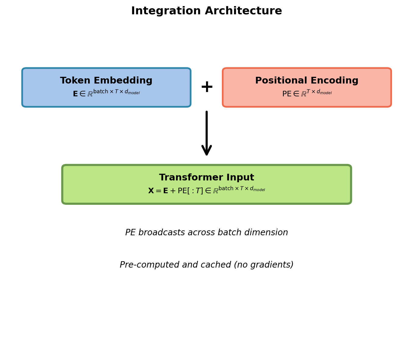
Approach:
\[\mathbf{X}_{input} = \mathbf{X}_{token} + \mathbf{X}_{position}\]
Both \(\in \mathbb{R}^{T \times d_{model}}\)
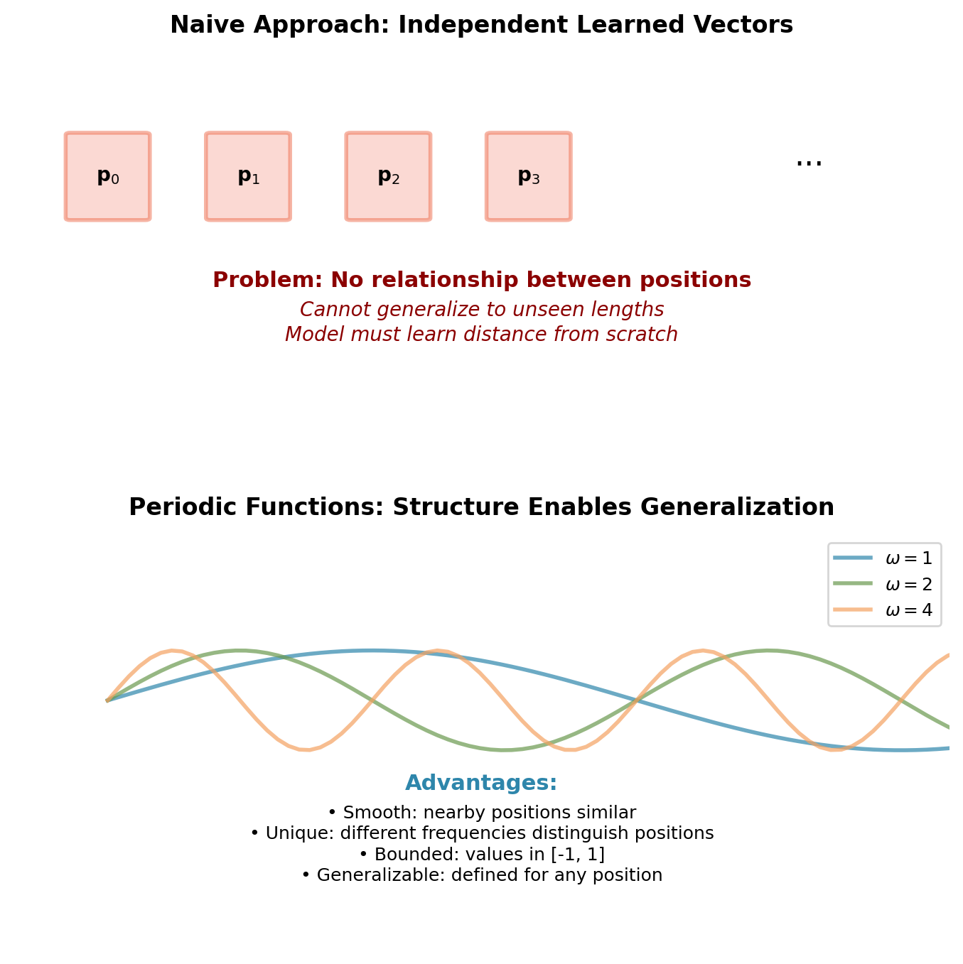
Why periodic functions?
Multiple sinusoids at different frequencies provide:
- Unique “fingerprint” for each position
- Smooth transitions between adjacent positions
- Bounded values that won’t dominate embeddings
- Natural extrapolation to arbitrary positions
Structure of Positional Encodings
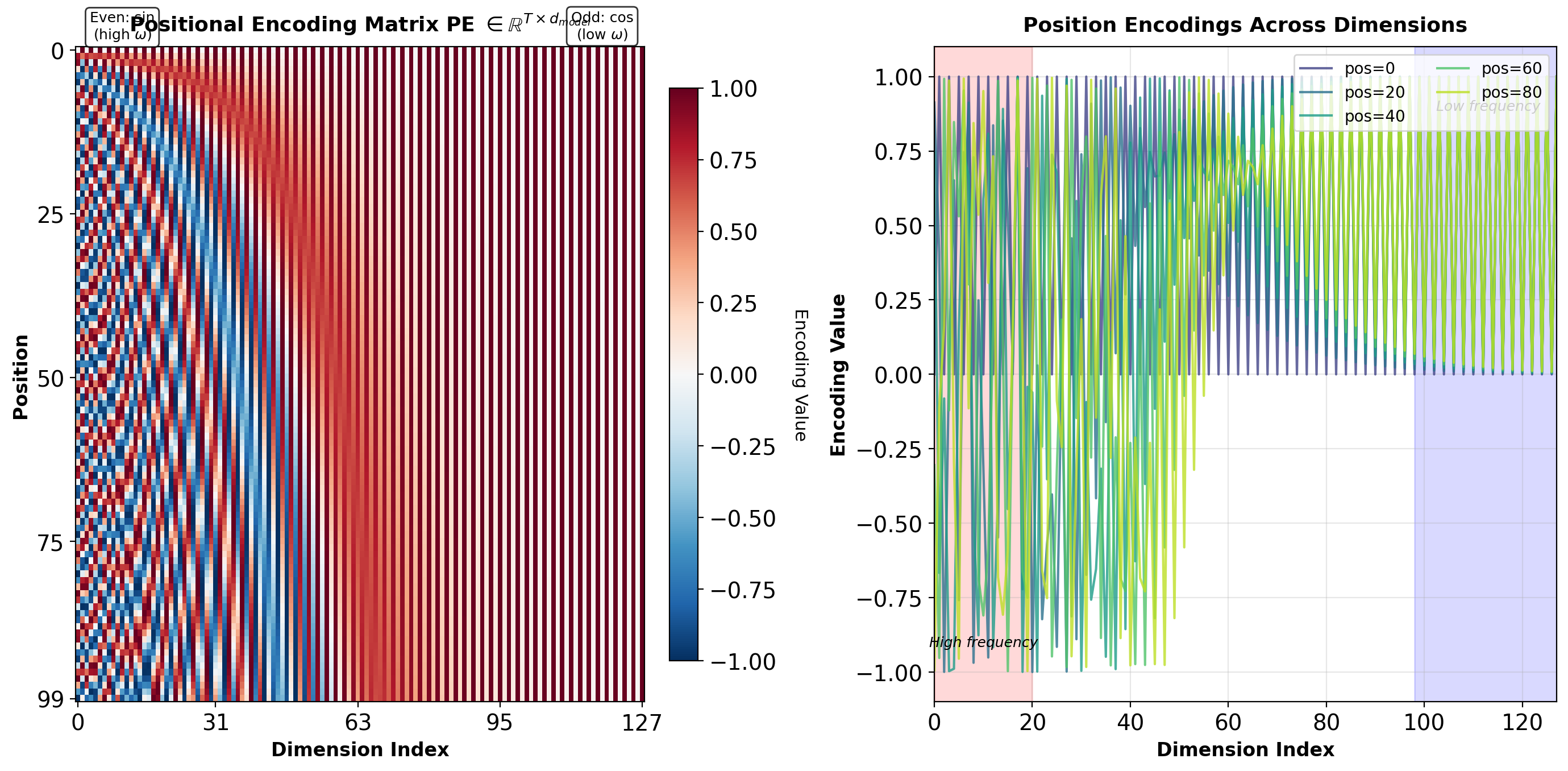
Interpretation:
- Rows (vertical axis): Position in sequence (\(0\) to \(T-1\))
- Columns (horizontal axis): Embedding dimension (\(0\) to \(d_{model}-1\))
- Left columns: High-frequency components (rapid oscillation with position)
- Right columns: Low-frequency components (slow variation with position)
Each position receives a unique \(d_{model}\)-dimensional vector.
Length Extrapolation Beyond Training
Sinusoidal encoding permits arbitrary sequence length:
- Formula defined for any position \(\text{pos} \in \mathbb{N}\)
- No architectural constraint on maximum length
- Can generate \(\text{PE}(\text{pos})\) for unseen positions
Empirical extrapolation performance (WMT’14 En→De, Transformer base):
| Train Length | Test Length | BLEU | Degradation |
|---|---|---|---|
| \(T \leq 512\) | 512 | 27.3 | — |
| \(T \leq 512\) | 768 | 26.0 | -1.3 |
| \(T \leq 512\) | 1024 | 25.0 | -2.3 |
| \(T \leq 512\) | 2048 | 22.7 | -4.6 |
Sources of degradation:
Attention weight distribution shift: Learned queries and keys optimized for positions seen during training. Softmax scores at unseen positions produce different distributions.
Relative magnitude changes: At position 1024, encoding magnitude remains bounded but relative to learned attention patterns, behaves differently than position 512.
No gradient signal: Training never updates parameters based on positions beyond \(T_{train}\). Model cannot learn appropriate behavior for extrapolation region.
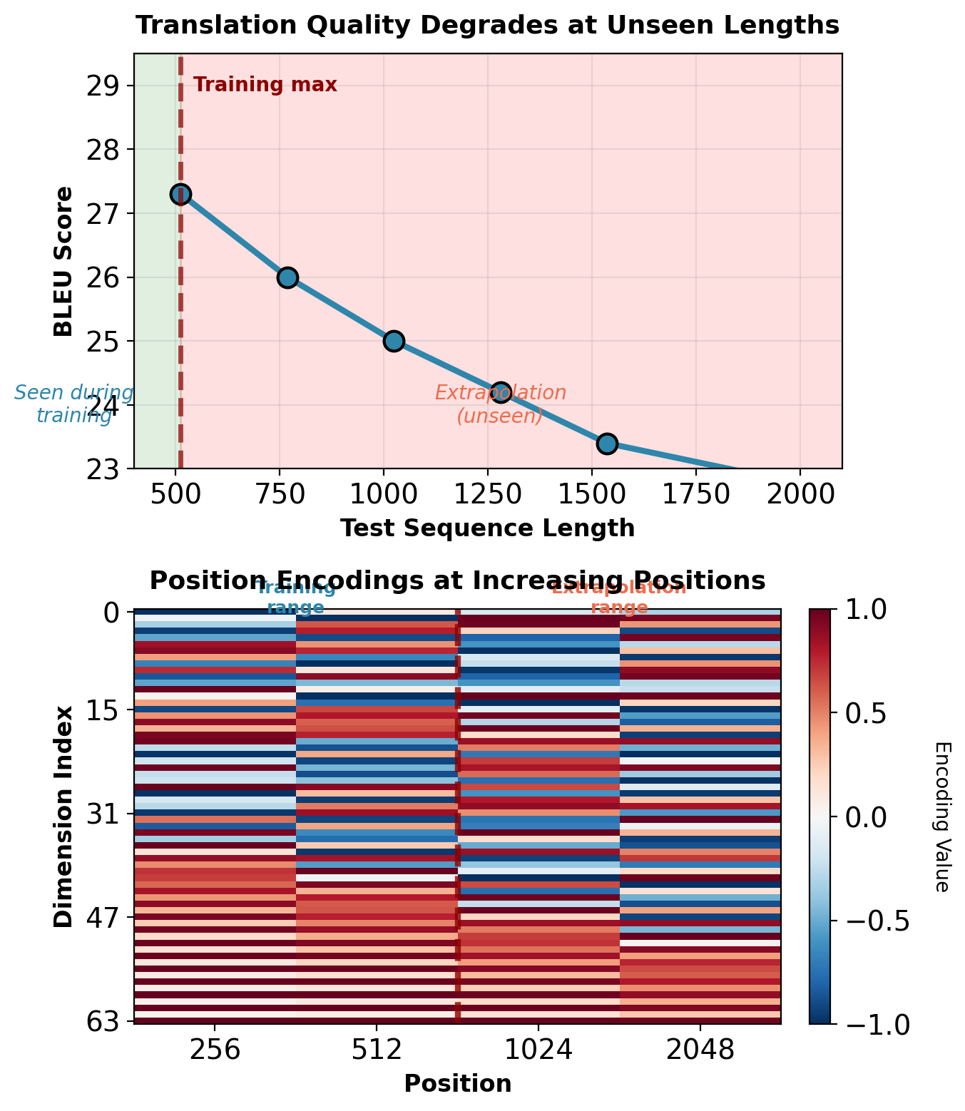
Practical implication: Training data must include sequence lengths matching deployment distribution. Sinusoidal encoding enables generation at any length but does not guarantee performance.
Implementation and Integration
Implementation:
import torch
import math

def get_positional_encoding(max_len, d_model):
    """
    Generate sinusoidal positional encodings.

    Returns:
        pe: Tensor [max_len, d_model]
    """
    pe = torch.zeros(max_len, d_model)
    position = torch.arange(0, max_len).unsqueeze(1)

    div_term = torch.exp(
        torch.arange(0, d_model, 2) *
        -(math.log(10000.0) / d_model)
    )

    pe[:, 0::2] = torch.sin(position * div_term)
    pe[:, 1::2] = torch.cos(position * div_term)

    return pe

# Usage
pos_enc = get_positional_encoding(5000, 512)

# Add to embeddings
# token_emb: [batch, seq_len, d_model]
input_emb = token_emb + pos_enc[:seq_len]
Key properties:
- Computed once at initialization
- No trainable parameters
- Sliced to match sequence length
- Broadcasts over batch dimension
- Values in \([-1, 1]\)
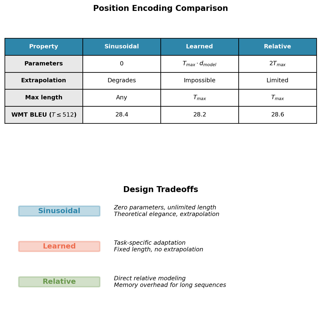
Alternative Position Encoding Approaches
Learned Positional Embeddings
Treat position as categorical variable with \(T_{max}\) classes. Learn embedding matrix \(\mathbf{P} \in \mathbb{R}^{T_{max} \times d_{model}}\) where position \(t\) maps to row \(\mathbf{P}[t]\).
Properties:
- Task-specific optimization during training
- Simpler implementation (standard embedding layer)
- Fixed maximum sequence length \(T_{max}\)
- Cannot generate encodings for positions \(> T_{max}\) (hard architectural limit)
Used in: BERT, GPT-2, GPT-3
Empirical performance: Comparable to sinusoidal within training length (WMT’14 En→De: 28.2 vs 28.4 BLEU at \(T \leq 512\))
Extrapolation: Architecturally impossible. Sequences longer than \(T_{max}\) require model retraining with larger embedding matrix.
Relative Position Encoding
Modify attention scores based on pairwise distance between positions.
\[e_{ij} = \mathbf{q}_i^T \mathbf{k}_j + a_{i-j}\]
where \(a_k\) is learned bias for offset \(k \in \{-T_{max}, \ldots, T_{max}\}\).
Properties:
- Direct encoding of relative distance
- \(2T_{max}\) learned parameters
- More interpretable position dependencies
Used in: Transformer-XL, T5
Other approaches:
- RoPE (Su et al., 2021): Rotary transformation applied to Q and K based on position
- ALiBi (Press et al., 2022): Linear biases added to attention scores
- No explicit encoding: Some architectures (Perceiver) use learned position queries
Performance differences minimal on standard benchmarks (\(<1\) BLEU). Architectural choice driven by sequence length requirements and computational constraints.
Encoder: Stack of Identical Layers
Architecture overview:
- \(N\) identical layers (typically \(N=6\))
- Each layer transforms \(\mathbb{R}^{T \times d_{model}} \to \mathbb{R}^{T \times d_{model}}\)
- Same dimension throughout entire stack
- No information bottleneck
Each layer contains:
- Multi-head self-attention sublayer
- Position-wise feed-forward network (FFN)
- Residual connection around each sublayer
- Layer normalization after each sublayer
Key principle:
- Same transformation applied at each position
- Weight sharing across positions (not across layers)
- Each layer refines representations from previous layer
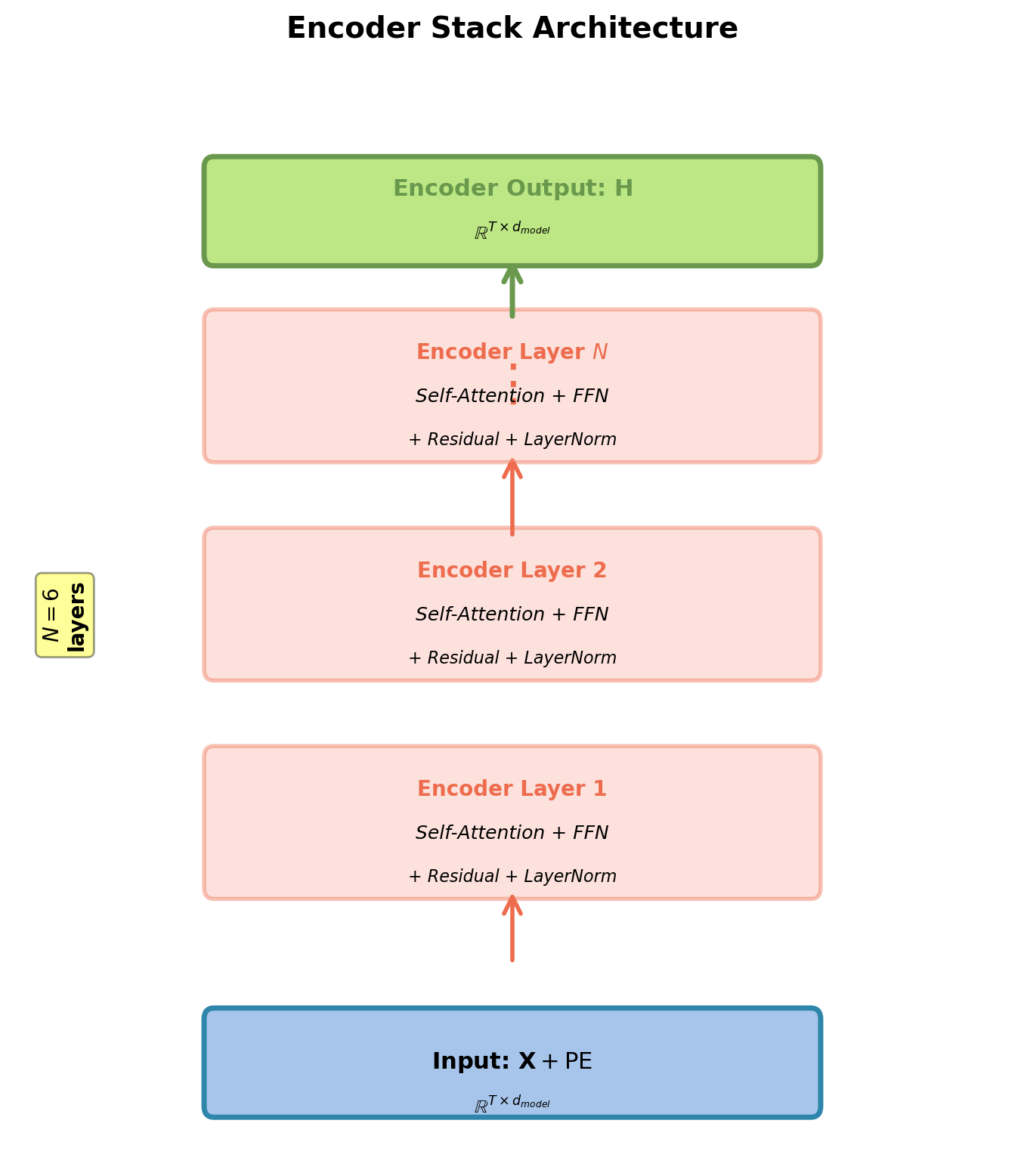
Dimension preservation: \(d_{model}\) constant throughout stack enables deep composition.
Encoder Layer Anatomy
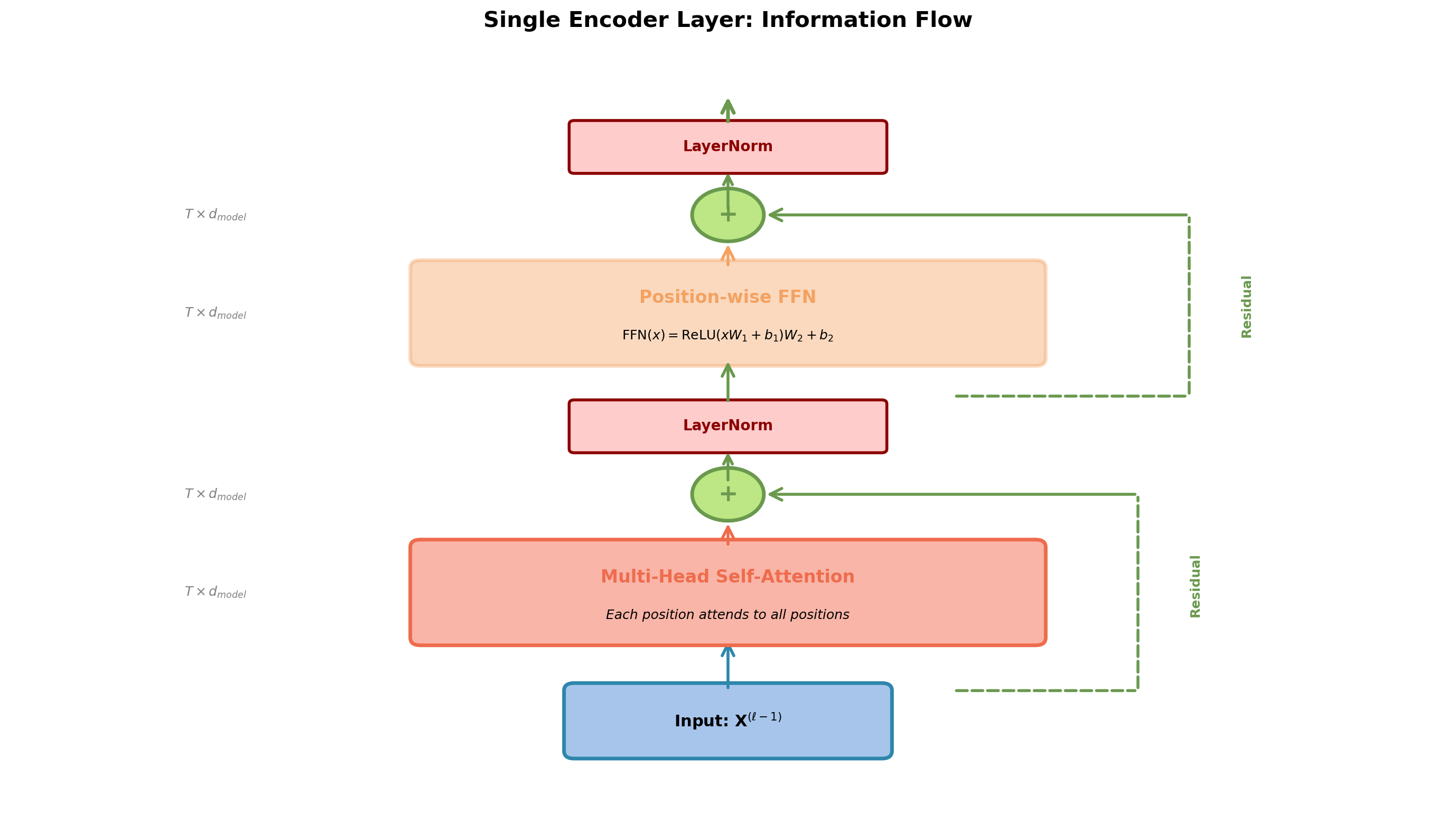
Two sublayers, each with residual connection and layer normalization.
Position-Wise Feed-Forward Networks
“Position-wise”: Same FFN applied independently to each position.
\[\text{FFN}(\mathbf{x}) = \text{ReLU}(\mathbf{x}\mathbf{W}_1 + \mathbf{b}_1)\mathbf{W}_2 + \mathbf{b}_2\]
Where:
- \(\mathbf{W}_1 \in \mathbb{R}^{d_{model} \times d_{ff}}\), typically \(d_{ff} = 4 \cdot d_{model}\)
- \(\mathbf{W}_2 \in \mathbb{R}^{d_{ff} \times d_{model}}\)
- Applied identically at each position
Why needed?
- Self-attention is linear in values: \(\mathbf{h}_i = \sum_j \alpha_{ij} \mathbf{v}_j\)
- FFN adds non-linearity and position-specific transformation
- Two linear layers with ReLU: increases capacity
Interpretation:
- Can be viewed as 1×1 convolution across sequence
- Hidden dimension \(d_{ff}\) provides bottleneck for feature mixing
- Parameters: \(2 \cdot d_{model} \cdot d_{ff}\) per layer
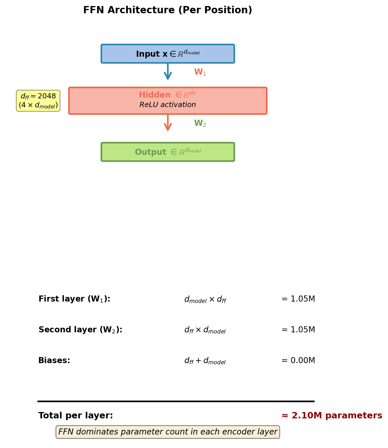
For \(d_{model}=512\), \(d_{ff}=2048\): FFN has ~2.1M parameters per layer.
Information Refinement Through Layers
Stacking creates hierarchical representations:
Lower layers (1-2):
- Local patterns and token relationships
- Syntactic dependencies (subject-verb)
- Nearby context integration
- High-frequency patterns
Middle layers (3-4):
- Phrasal structures
- Constituent boundaries
- Medium-range dependencies
- Compositional semantics
Upper layers (5-6):
- Abstract semantic features
- Discourse relationships
- Long-range dependencies
- Task-specific representations
Empirical observation:
Each layer specializes without supervision, patterns emerge from task optimization.
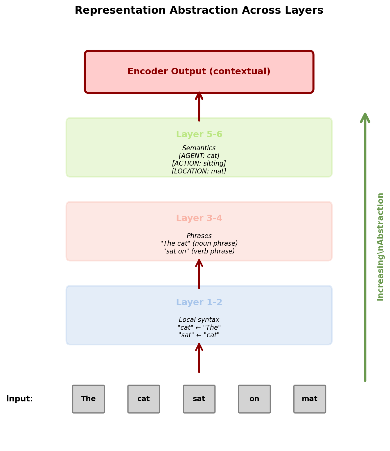
Each position’s representation becomes increasingly context-aware and abstract.
Receptive Field Growth
After \(L\) layers, each position has accessed:
- Direct connections to all \(T\) positions at every layer
- Information flows through \(L\) transformation stages
- Effective receptive field: Full sequence from layer 1
Contrast with CNNs:
- CNN: Receptive field grows linearly/polynomially with depth
- 3×3 convolution: Radius grows by 1 per layer
- Need many layers to see full sequence
Transformer advantage:
- Global receptive field immediately (layer 1)
- Each layer adds refinement, not scope
- Enables modeling of arbitrarily long-range dependencies
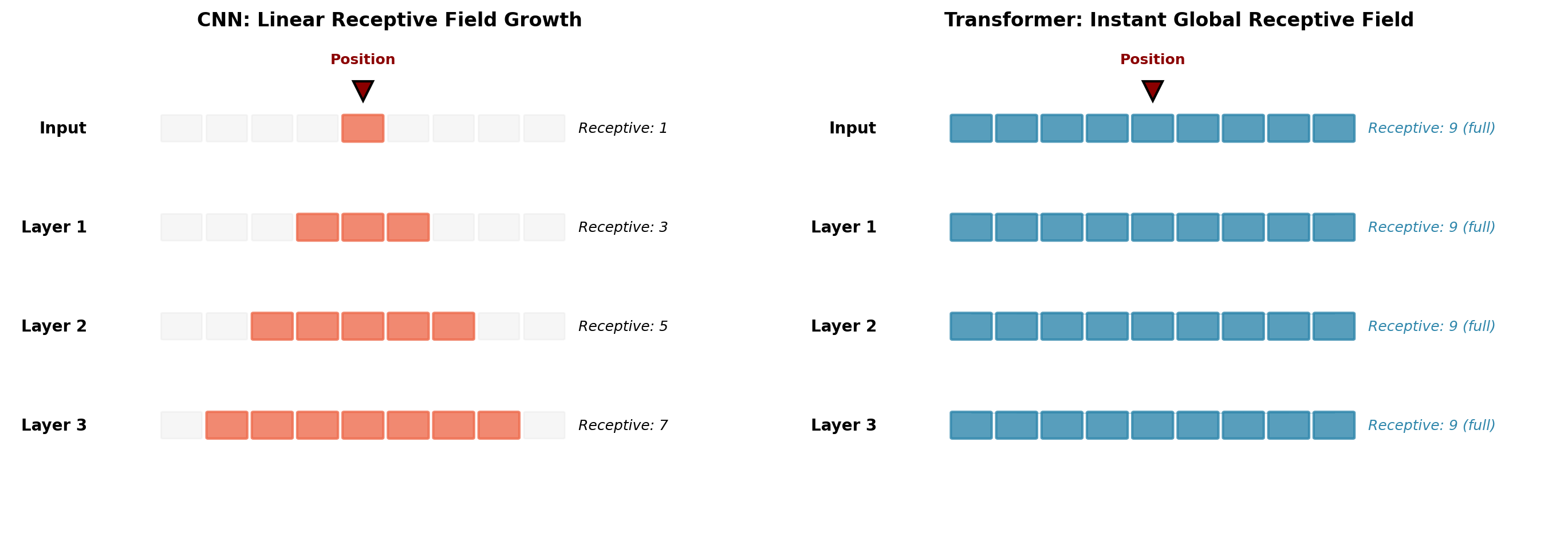
Transformer sees full sequence at every layer. CNN must stack many layers to achieve same scope.
Residual Connections: Enabling Deep Networks
Standard layer transformation:
\[\mathbf{x}^{(\ell)} = F(\mathbf{x}^{(\ell-1)})\]
Gradient through \(L\) layers: \[\frac{\partial \mathcal{L}}{\partial \mathbf{x}^{(0)}} = \frac{\partial \mathcal{L}}{\partial \mathbf{x}^{(L)}} \prod_{\ell=1}^L \frac{\partial F^{(\ell)}}{\partial \mathbf{x}^{(\ell-1)}}\]
Problem: Product of Jacobians causes vanishing/exploding gradients.
Residual connection:
\[\mathbf{x}^{(\ell)} = \mathbf{x}^{(\ell-1)} + F(\mathbf{x}^{(\ell-1)})\]
Key property: Identity path bypasses transformation.
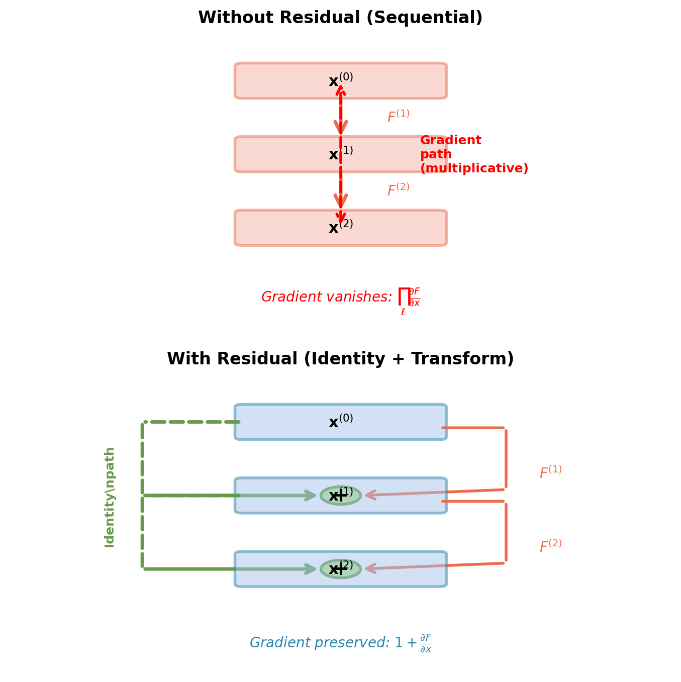
Identity path ensures gradient can always flow through the network.
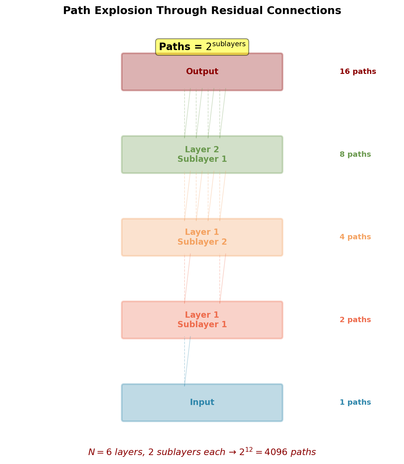
Path Explosion in Deep Transformers
Each encoder layer has 2 residual connections:
- Around self-attention
- Around feed-forward network
For \(N\) layers:
- Total sublayers: \(2N\)
- Number of possible paths: \(2^{2N}\)
6-layer transformer:
- Paths: \(2^{12} = 4096\) different routes from input to output
- Each path is a composition of identity and transformation
- Gradient = average over all paths
Ensemble interpretation:
- Each path acts like a separate model
- Network learns features that work across many paths
- Robust to individual path failures
- Explains training stability of very deep transformers
Exponential path count enables very deep networks (50+ layers) without gradient issues.
Batch Normalization Failure for Sequences
Batch normalization computes statistics across batch dimension.
For minibatch \(\mathcal{B} = \{x^{(1)}, \ldots, x^{(B)}\}\) and feature \(j\):
\[\mu_j = \frac{1}{B}\sum_{b=1}^B x_j^{(b)}, \quad \sigma_j^2 = \frac{1}{B}\sum_{b=1}^B (x_j^{(b)} - \mu_j)^2\]
Normalize: \(\hat{x}_j^{(b)} = \frac{x_j^{(b)} - \mu_j}{\sqrt{\sigma_j^2 + \epsilon}}\)
Works for CNNs: Each feature has consistent meaning across spatial positions and samples.
Fails for sequences:
- Variable length: \(T\) varies across batch
- Position-dependent distributions: Token at position 5 has different statistics than position 50
- Batch size sensitivity: Small \(B\) → unreliable statistics
- Inference mismatch: Single-sample inference uses running statistics from training
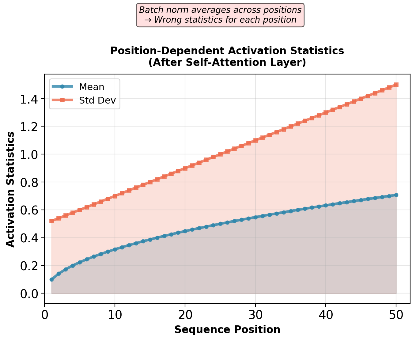
Position-dependent statistics cannot be captured by batch-level normalization.
Layer Normalization Solution
Normalize across feature dimension for each sample and position independently:
\[\mu^{(t)} = \frac{1}{d}\sum_{i=1}^d x_i^{(t)}, \quad \sigma^{2(t)} = \frac{1}{d}\sum_{i=1}^d (x_i^{(t)} - \mu^{(t)})^2\]
\[\text{LayerNorm}(\mathbf{x}^{(t)}) = \gamma \odot \frac{\mathbf{x}^{(t)} - \mu^{(t)}}{\sqrt{\sigma^{2(t)} + \epsilon}} + \beta\]
where \(\gamma, \beta \in \mathbb{R}^d\) are learned per-feature scale and shift.
Properties:
- No batch statistics: Each sample normalized independently
- No position coupling: Each position has own \(\mu, \sigma\)
- Inference = Training: No running average needed
- Sequence length invariant: Works for any \(T\)
Computational cost: \(O(d)\) per position, negligible compared to attention \(O(T \cdot d)\).
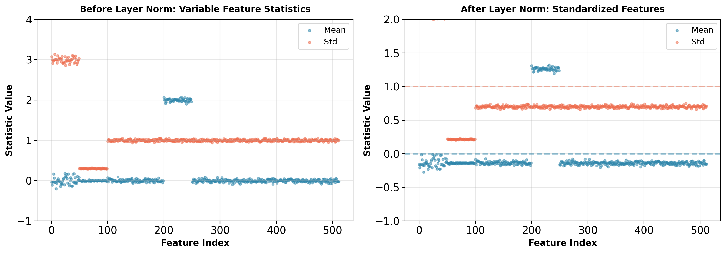
Layer normalization standardizes each position independently, removing scale variations across features.
Training Dynamics: Gradient Norms Across Depth
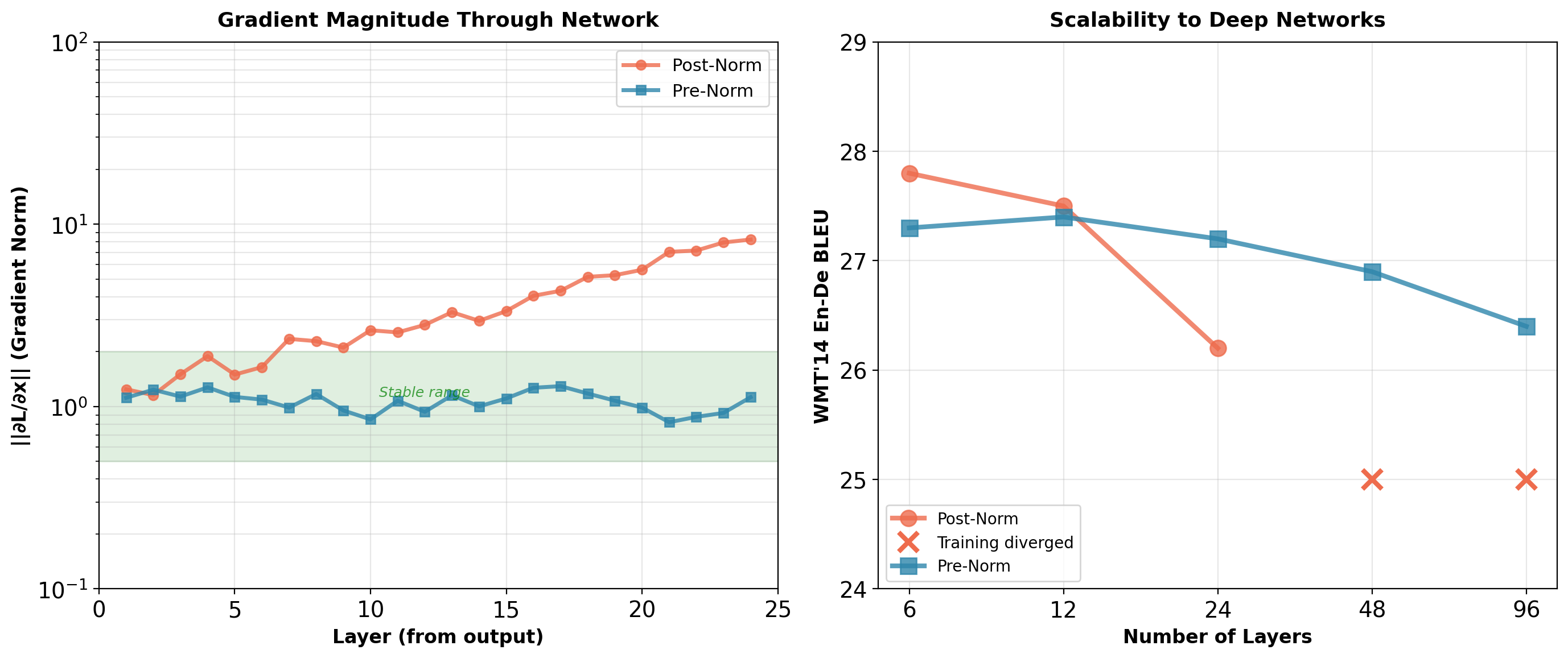
WMT’14 En-De results: Post-norm optimal at 6 layers (27.8 BLEU), fails at 48+ layers. Pre-norm maintains training stability across all depths, with 6-layer slightly lower (27.3 BLEU, -0.5).
Representation Norm Growth
Without normalization in residual path, representation norms accumulate:
After \(L\) layers with residual connections: \[\mathbf{x}^{(L)} = \mathbf{x}^{(0)} + \sum_{\ell=1}^L F^{(\ell)}(\cdot)\]
Expected norm growth: \(\|\mathbf{x}^{(L)}\| \approx \sqrt{L} \cdot \|\mathbf{x}^{(0)}\|\) (random walk in high dimensions).
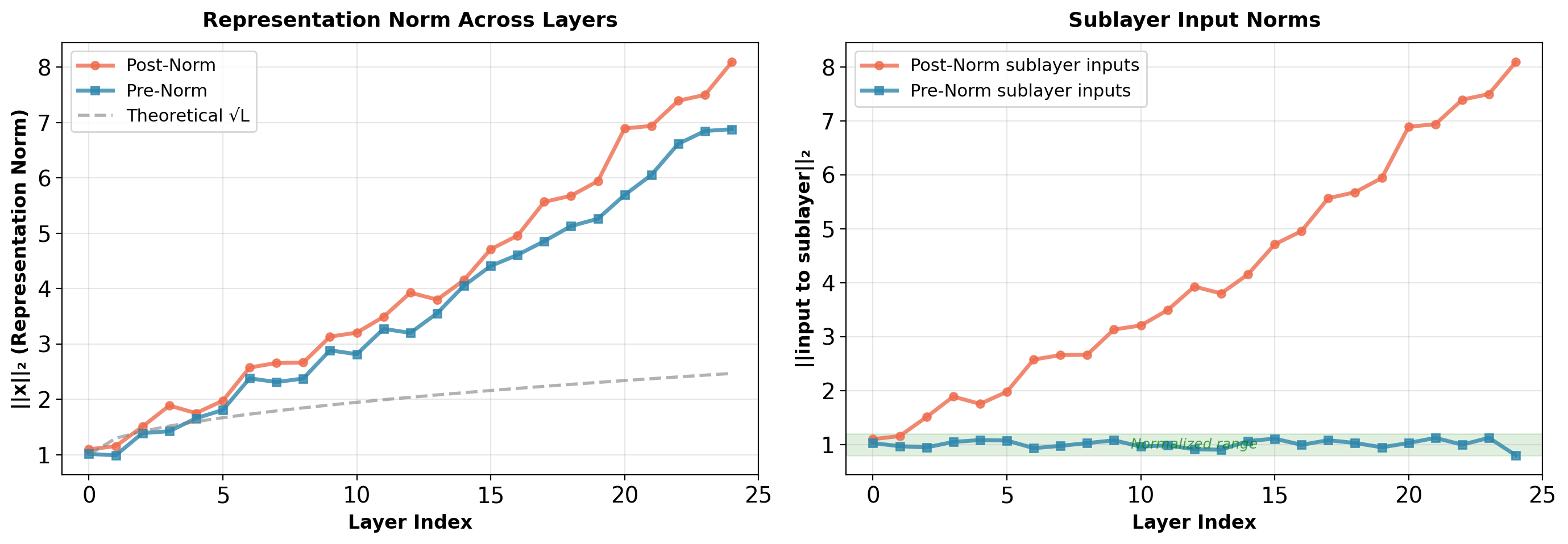
Pre-norm advantage: Sublayers always operate on normalized inputs (‖input‖ ≈ 1), preventing sensitivity to depth. Residual path accumulates unnormalized updates, but this doesn’t affect gradient flow through identity connection.
Decoder Architecture: Three Sublayers
Decoder layer structure:
Each of \(N\) layers (typically \(N=6\)) contains three sublayers:
- Masked self-attention
- Attends to previous positions in target sequence
- Causal constraint: Position \(t\) cannot see positions \(> t\)
- Encoder-decoder cross-attention
- Query from decoder, Keys/Values from encoder output
- Attends to full source sequence (no masking)
- Position-wise FFN
- Same as encoder FFN
Each sublayer has residual connection and layer normalization.
Critical difference from encoder: Decoder must maintain causality for autoregressive generation.
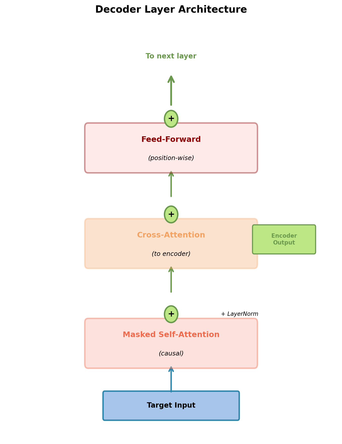
Three sublayers process target sequence with access to encoder representations.
Causal Masking: Preventing Information Leakage
Autoregressive generation requires: \(p(y_t | y_{<t}, \mathbf{x})\)
Position \(t\) can only depend on positions \(\{1, 2, \ldots, t\}\), not future positions \(\{t+1, \ldots, T\}\).
During training:
- Have full target sequence available
- Must simulate sequential generation
- Prevent attention to future positions
Masking mechanism:
Attention scores before softmax: \(\mathbf{S} = \frac{\mathbf{QK}^T}{\sqrt{d_k}} \in \mathbb{R}^{T \times T}\)
Apply mask \(\mathbf{M}\) where \(M_{ij} = \begin{cases} 0 & \text{if } i \geq j \\ -\infty & \text{if } i < j \end{cases}\)
Masked scores: \(\tilde{\mathbf{S}} = \mathbf{S} + \mathbf{M}\)
After softmax: Future positions have weight 0.
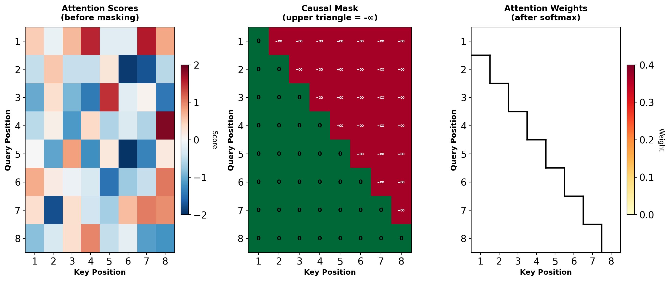
Upper triangle (future) forced to zero probability after softmax.
Training Efficiency: Parallel Computation with Masking
Masking enables parallel training on full sequence.
RNN decoder training:
- Generate \(y_1\), then \(y_2\), …, then \(y_T\) sequentially
- Cannot parallelize: \(y_t\) requires \(y_{t-1}\)
- \(T\) sequential forward passes
Masked transformer decoder training:
- Process all positions simultaneously
- Masking enforces causal dependency implicitly
- Loss computed at all positions in parallel: \(\mathcal{L} = \sum_{t=1}^T \log p(y_t | y_{<t}, \mathbf{x})\)
Training speedup: Up to \(100\times\) for long sequences (parallel vs sequential).
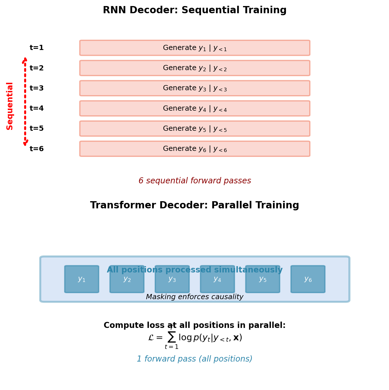
Parallel processing during training compensates for quadratic attention cost: up to 100× faster than RNN despite \(O(T^2)\) complexity.
Inference: Sequential Generation with KV Caching
At inference, generation is sequential:
- Generate \(y_1 \sim p(\cdot | \text{START}, \mathbf{x})\)
- Generate \(y_2 \sim p(\cdot | y_1, \mathbf{x})\)
- Continue until END token or max length
Naive approach: Recompute attention for all previous tokens at each step.
For position \(t\): Process tokens \(\{y_1, \ldots, y_t\}\) through decoder.
Computational cost: \(O(T^2)\) attention operations for sequence of length \(T\).
Optimization: KV caching
Keys and values from previous positions don’t change. Cache them:
- At step \(t-1\): Store \(\mathbf{K}_{<t}, \mathbf{V}_{<t}\)
- At step \(t\): Compute only \(\mathbf{k}_t, \mathbf{v}_t\) from \(y_t\)
- Concatenate: \(\mathbf{K}_{\leq t} = [\mathbf{K}_{<t}; \mathbf{k}_t]\)
- Attention: \(\mathbf{h}_t = \sum_{j=1}^t \alpha_{tj} \mathbf{v}_j\)
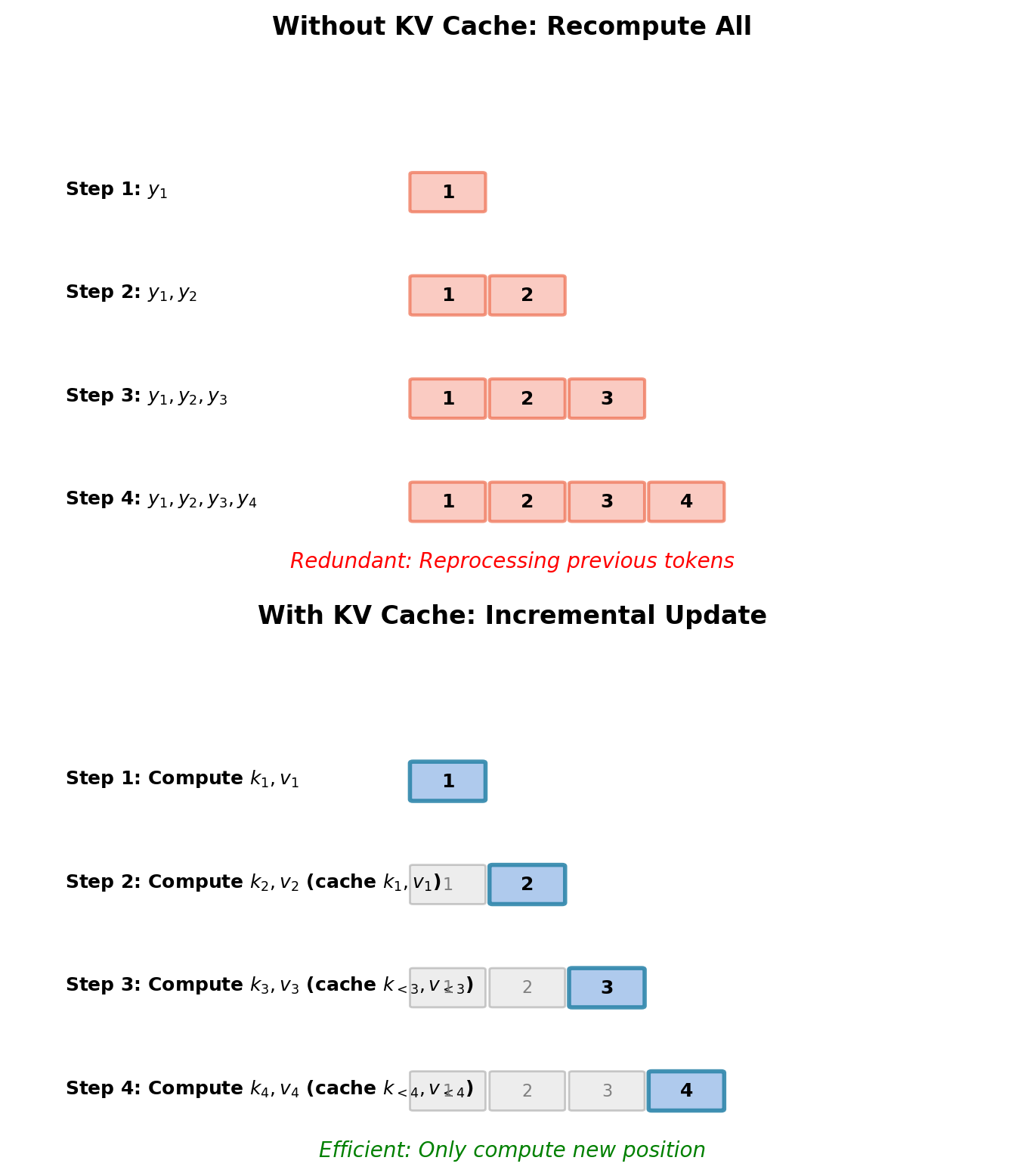
Memory-speed tradeoff: Store \(O(L \times T \times d)\) cached keys/values (where \(L\) = number of layers), reduce computation from \(O(T^2)\) to \(O(T)\) per generation step.
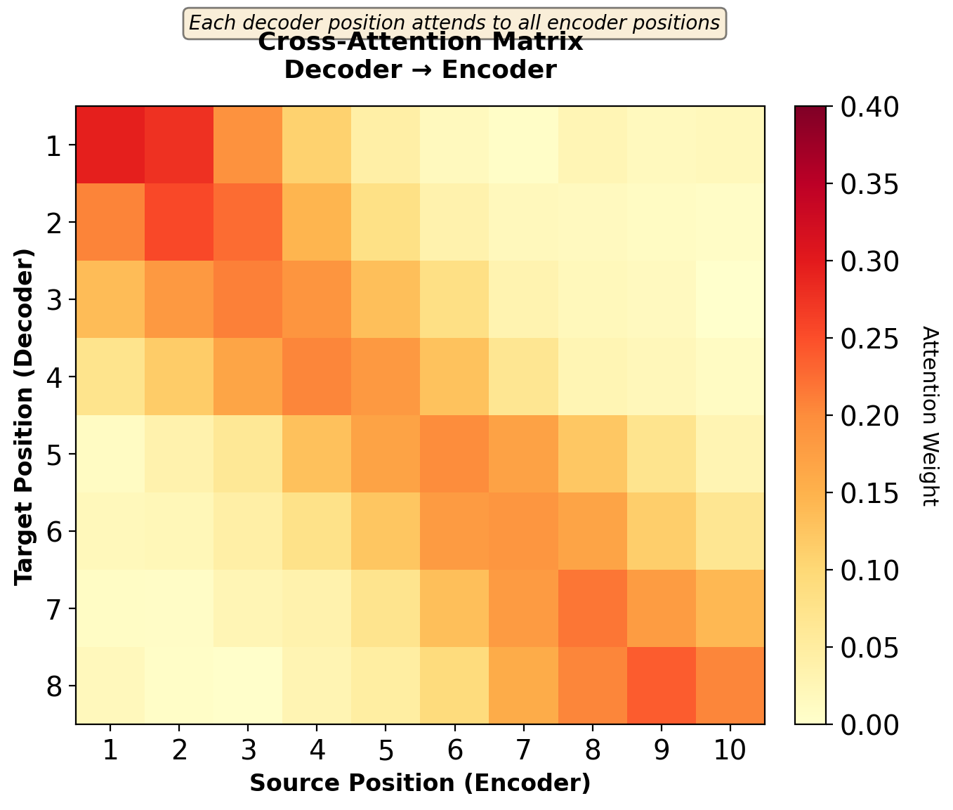
Encoder-Decoder Cross-Attention
Cross-attention sublayer:
- Query: From decoder (previous sublayer output)
- Keys, Values: From encoder output (final encoder layer)
- No masking: Decoder can attend to entire source sequence
\[\text{CrossAttention}(\mathbf{Q}_{dec}, \mathbf{K}_{enc}, \mathbf{V}_{enc})\]
where:
- \(\mathbf{Q}_{dec} = \mathbf{X}_{dec} \mathbf{W}^Q \in \mathbb{R}^{T_t \times d_k}\)
- \(\mathbf{K}_{enc} = \mathbf{H}_{enc} \mathbf{W}^K \in \mathbb{R}^{T_s \times d_k}\)
- \(\mathbf{V}_{enc} = \mathbf{H}_{enc} \mathbf{W}^V \in \mathbb{R}^{T_s \times d_v}\)
Attention matrix: \(\mathbb{R}^{T_t \times T_s}\) (target positions × source positions)
This is the same attention mechanism from Lecture 05, now operating on transformer representations.
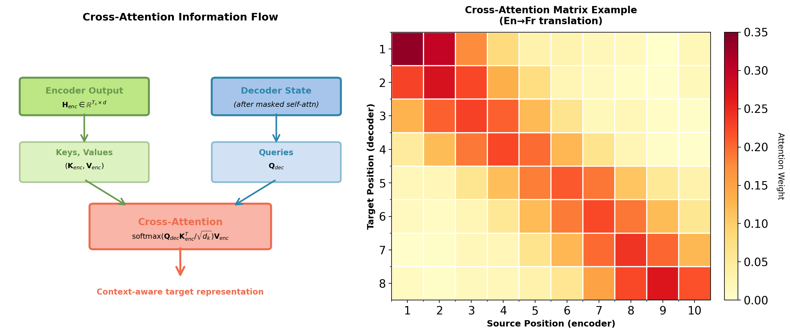
Each decoder position attends to full source sequence to retrieve relevant information for generation.
Complete Transformer System
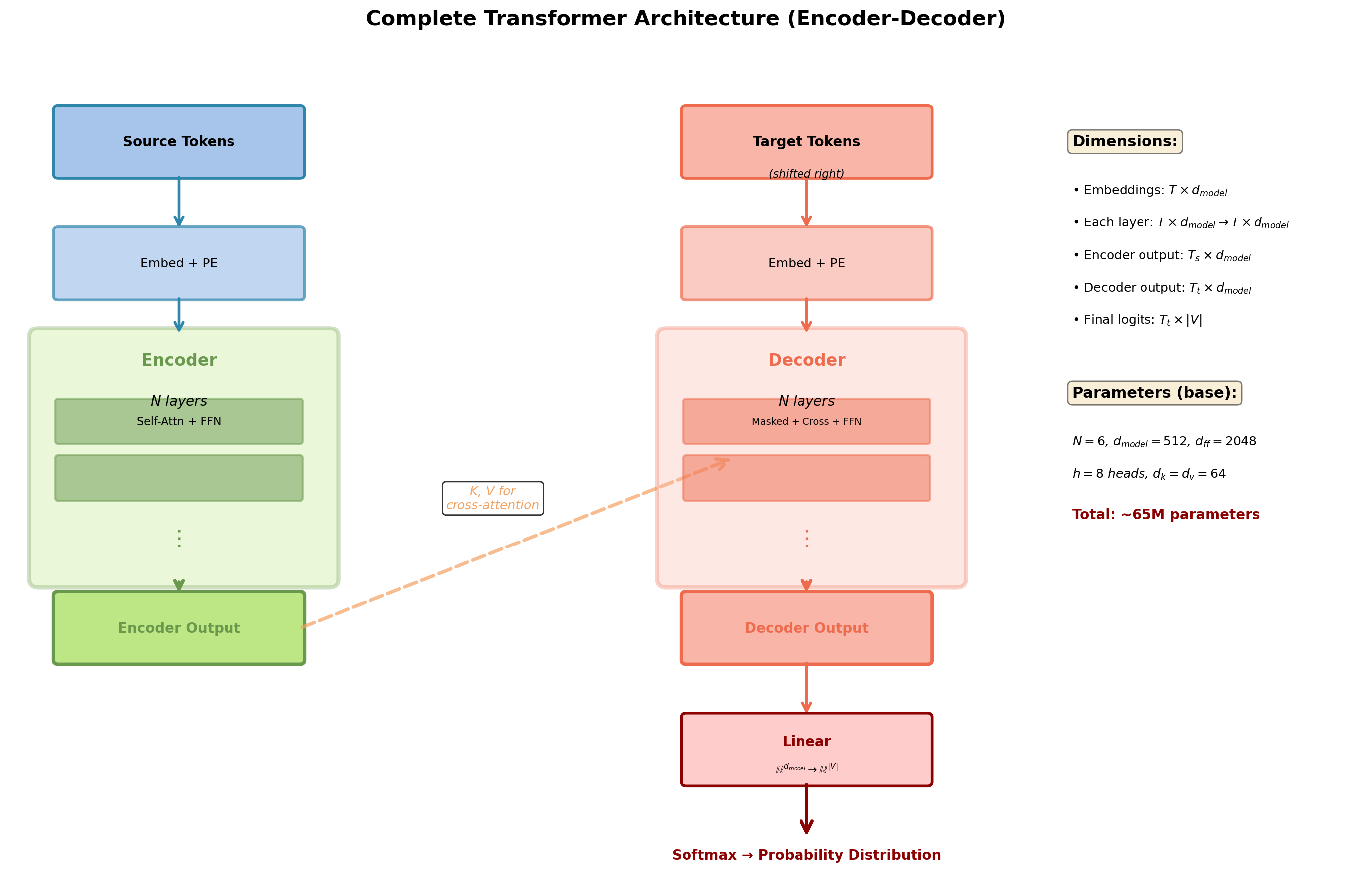
Standard transformer: 6-layer encoder, 6-layer decoder, multi-head self-attention and cross-attention, position-wise FFN with residuals and layer norm at each sublayer.
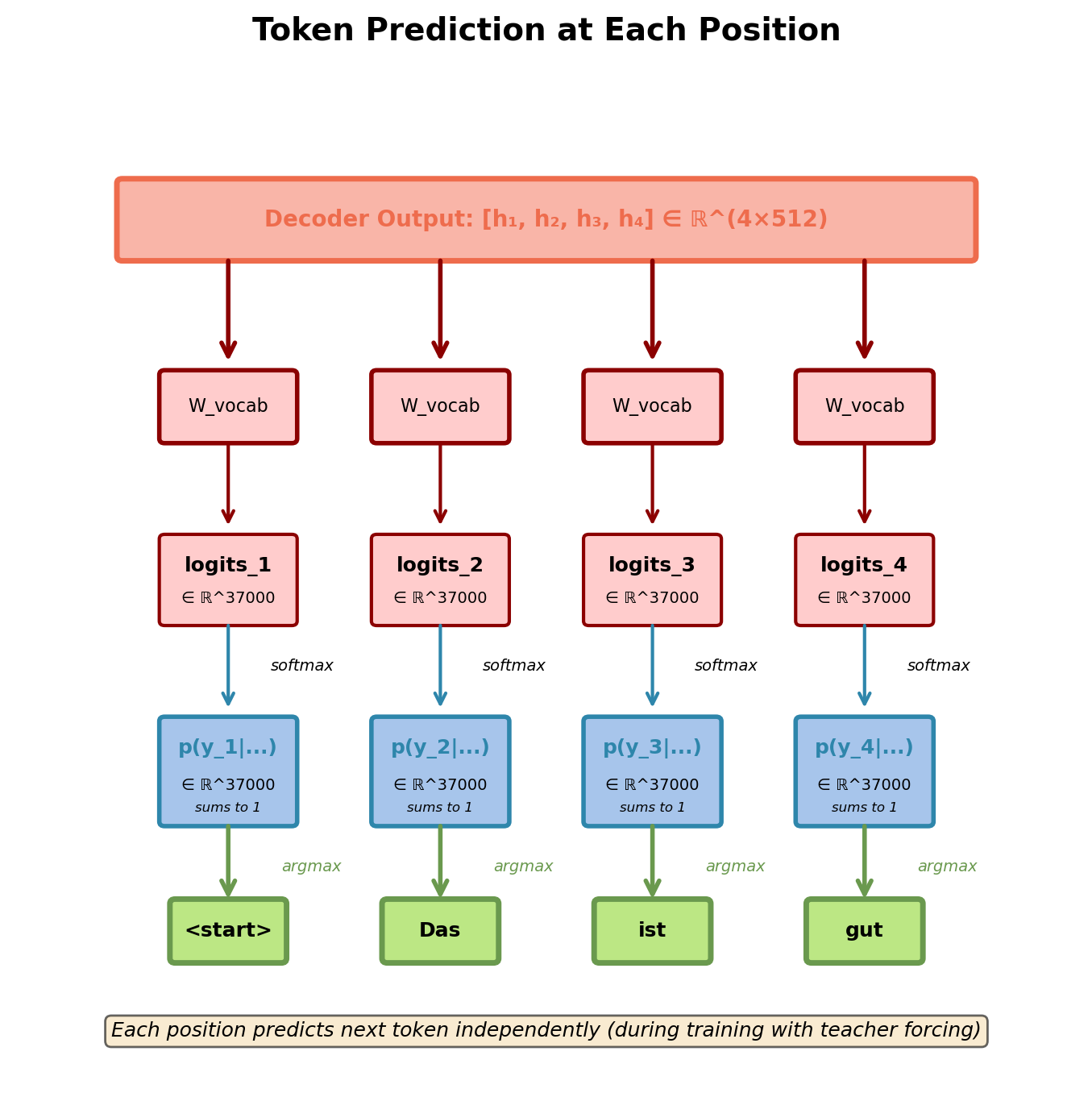
Output Projection: From Representations to Tokens
Decoder produces contextualized representations ∈ ℝ^(T×d_model)
Output layer maps to vocabulary:
\[\mathbf{logits} = \mathbf{H}_{decoder}\mathbf{W}_{vocab}\]
Where W_vocab ∈ ℝ^(d_model × |V|) projects each position to vocabulary size.
Per-position softmax:
\[p(y_t | y_{<t}, \mathbf{x}) = \text{softmax}(\mathbf{logits}_t) \in \mathbb{R}^{|V|}\]
Each decoder position produces probability distribution over vocabulary.
For translation (WMT’14 En-De):
- Vocabulary size: |V| = 37,000 (BPE)
- Output projection: 512 × 37,000 = 19M parameters
- Softmax computed independently for each position
Training: Cross-entropy loss at each position \[\mathcal{L} = -\sum_{t=1}^T \log p(y_t^* | y_{<t}, \mathbf{x})\]
where y_t^* is ground truth token.
Output projection weight matrix often tied with input embeddings (W_vocab^T = W_embed), reducing parameters by |V| × d_model.
System Resources: Parameters and Memory
Parameter count (base config: \(N=6\), \(d_{model}=512\), \(d_{ff}=2048\)):
- Embeddings: 32M (vocabulary × \(d_{model}\))
- Encoder: 31M (6 layers × attention + FFN)
- Decoder: 37M (6 layers × 3 sublayers)
- Total: ~65M parameters
Scaling:
- Base (\(d_{model}=512\)): 65M parameters
- Big (\(d_{model}=1024\)): 213M parameters
FFN layers dominate: \(2 \times d_{model} \times d_{ff}\) per layer.
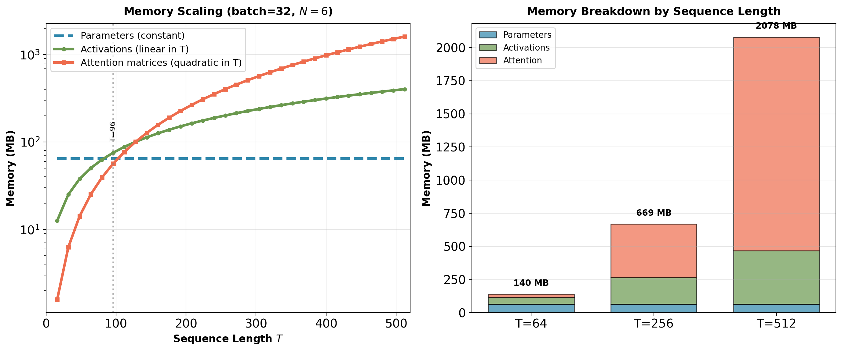
Memory scaling with sequence length:
Parameters are constant (65MB), but activations and attention scale with \(T\):
- Activations: \(O(T)\) - linear in sequence length
- Attention matrices: \(O(T^2)\) - quadratic bottleneck
Crossover: Attention memory dominates when \(T > 256\).
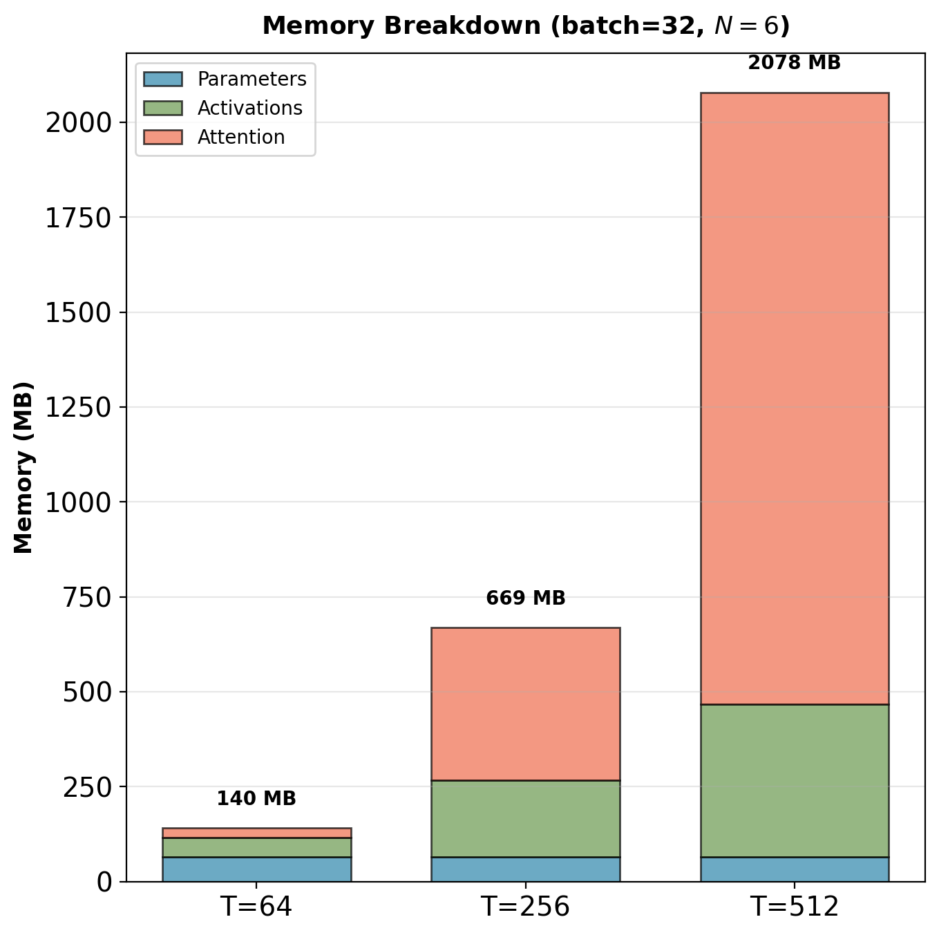
At \(T=512\), batch=32: Attention matrices require 4GB, dominating total memory. Parameters (65MB) negligible.
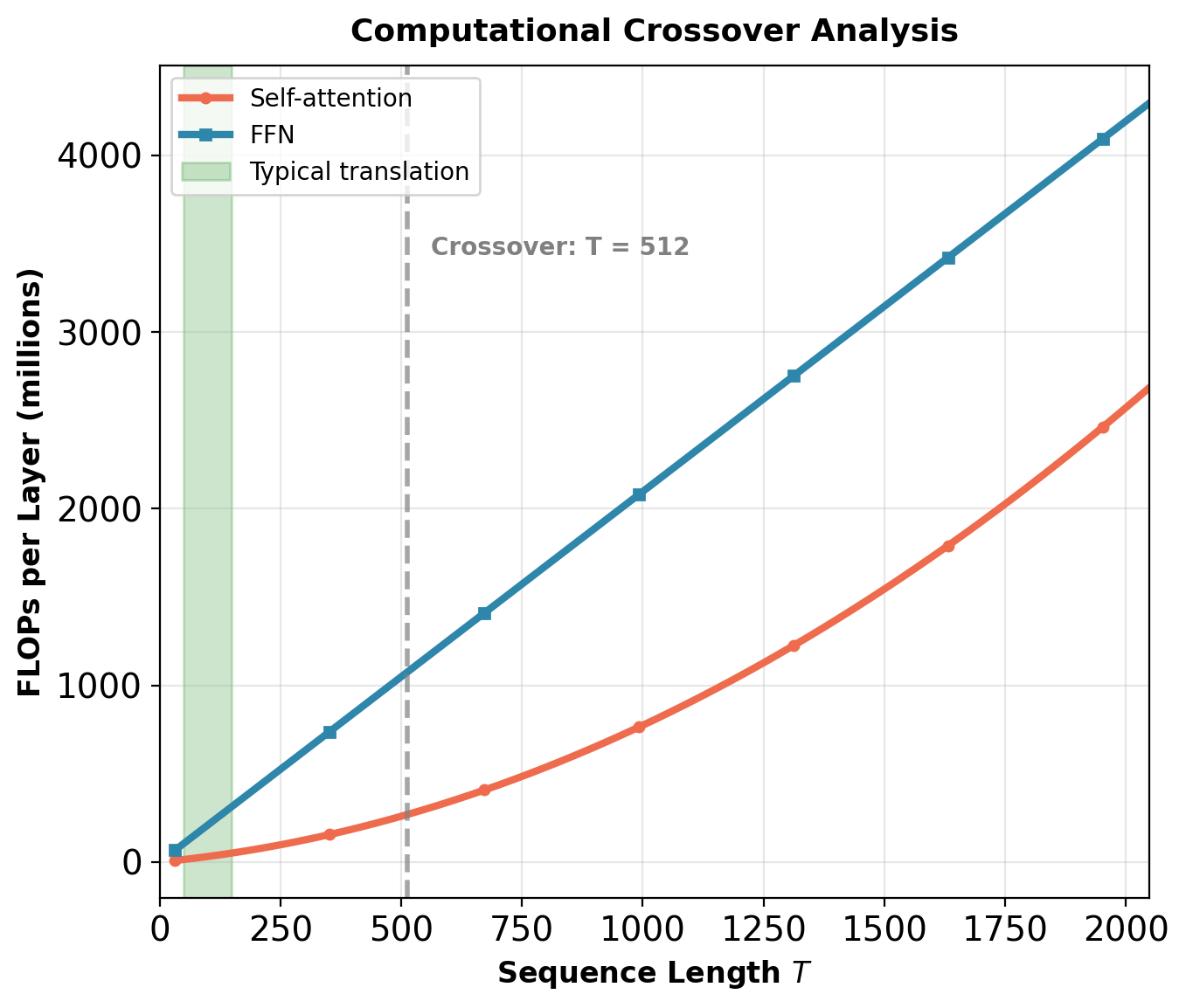
Computational Complexity: When Does Quadratic Cost Matter?
Per-layer complexity:
- Self-attention: \(O(T^2 \cdot d_{model} + T \cdot d_{model}^2)\)
- FFN: \(O(T \cdot d_{model} \cdot d_{ff})\) where \(d_{ff} = 4 d_{model}\)
Crossover point: Self-attention dominates when \(T^2 d_{model} > T d_{model}^2\), i.e., when \(T > d_{model}\).
For \(d_{model} = 512\):
- \(T < 512\): FFN dominates (typical for translation)
- \(T > 512\): Self-attention dominates (long documents)
Concrete example (\(N=6\), \(d=512\), \(T=100\)):
- Self-attention: 61M FLOPs
- FFN: 314M FLOPs
FFN uses 5× more computation than attention for translation.
Reality: The “quadratic bottleneck” narrative is misleading for typical NLP tasks. Attention becomes the computational bottleneck only for very long sequences (\(T > 512\)).
Gradient Flow: Exponential Path Count
Key observation: For \(T=512\), attention matrices require 4GB memory (batch=32), dominating total memory. Parameters (65MB) negligible by comparison.
Gradient Flow: Exponential Path Count
Each encoder/decoder layer has 2-3 residual connections:
- Encoder layer: 2 residuals (self-attention, FFN)
- Decoder layer: 3 residuals (masked self-attention, cross-attention, FFN)
Total gradient paths from output to input:
For \(N\) encoder layers and \(N\) decoder layers: \[\text{Paths} = 2^{2N} \times 2^{3N} = 2^{5N}\]
For \(N=6\): \(2^{30} \approx 1\) billion paths.
Gradient at input is average over all paths.
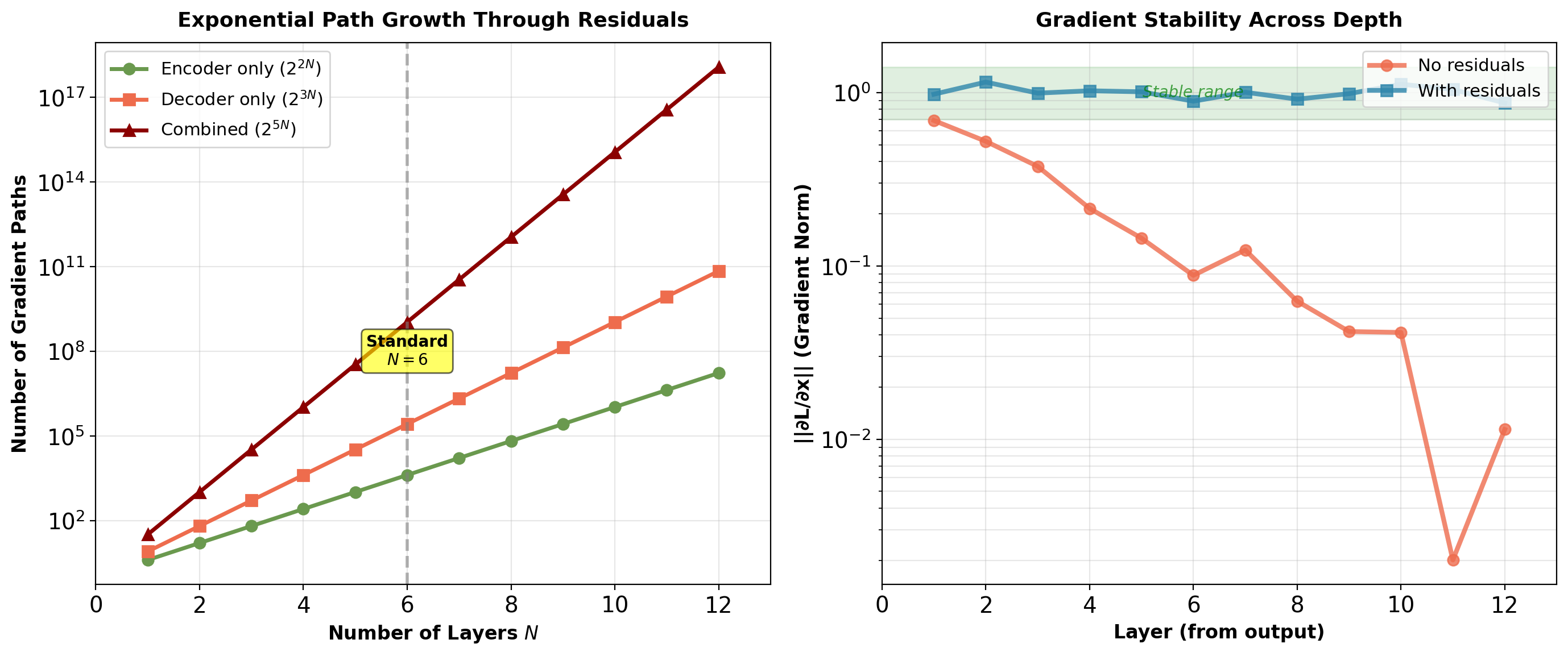
Ensemble interpretation: Gradient is averaged over \(2^{5N}\) paths. Individual path failures don’t prevent training as long as sufficient paths remain viable. The exponential number of viable paths ensures training stability in deep transformers.
Transformers Fail with Standard Learning Rate Schedules
Standard approach for neural networks:
- Constant learning rate (e.g., 0.001)
- Or: Start high, decay gradually
- Works for CNNs, RNNs, MLPs
Transformers trained this way:
- Loss explodes within 100-500 steps
- Gradients grow to \(10^6\)-\(10^8\) magnitude
- NaN values appear in attention weights
- Training diverges completely
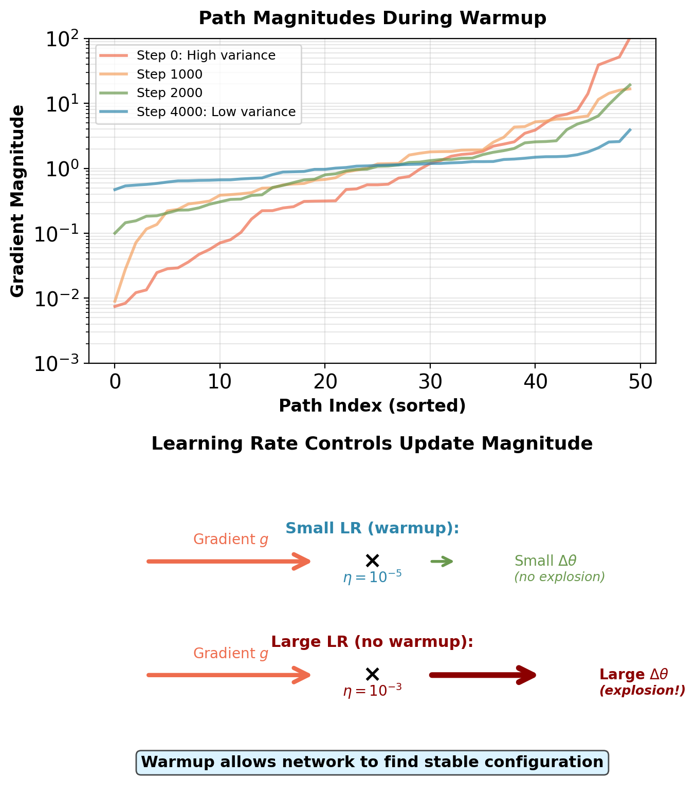
Standard solution: Learning rate warmup
- Start at learning rate ≈ 0
- Gradually increase to target over first 4,000-8,000 steps
- Then apply standard decay schedule
- Without warmup: Training typically diverges
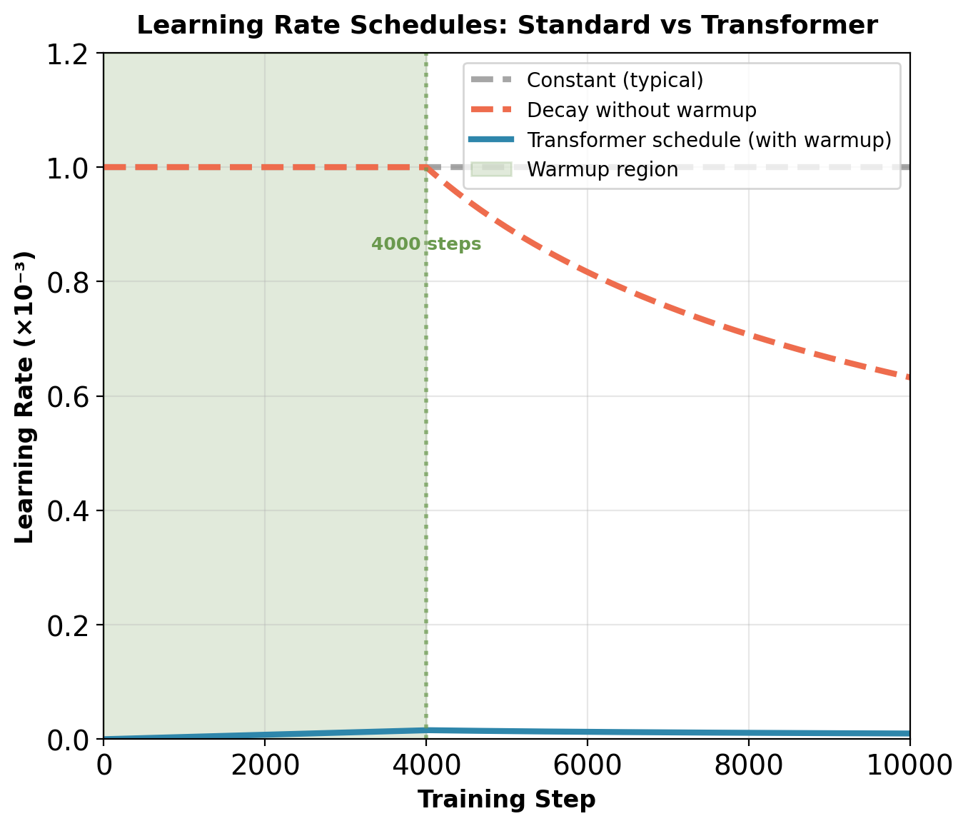
Transformer learning rate schedule: \(\text{lr} = d_{\text{model}}^{-0.5} \cdot \min(\text{step}^{-0.5}, \text{step} \cdot \text{warmup\_steps}^{-1.5})\)
Training Instability: Loss Explosion Without Warmup
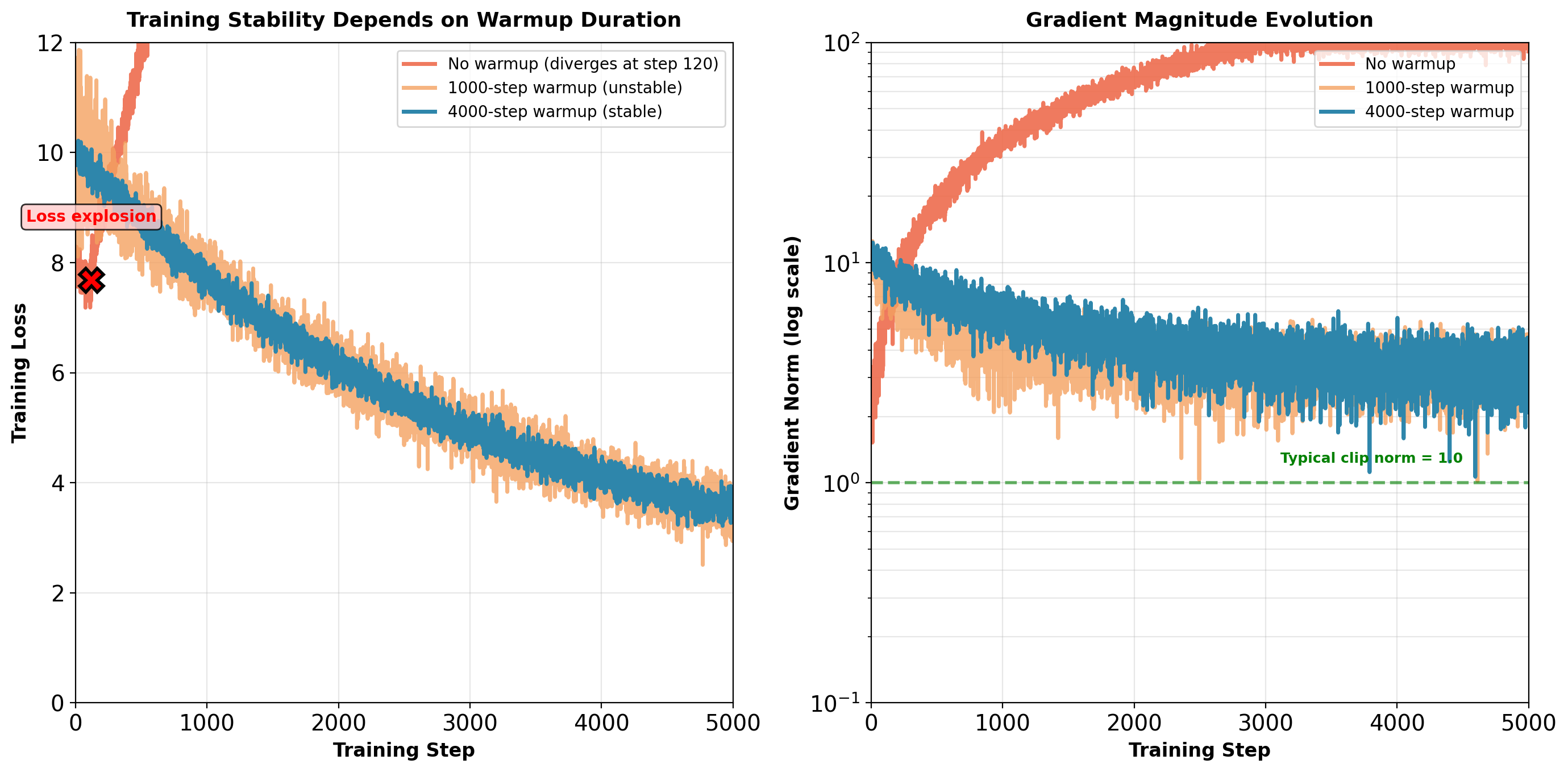
Without warmup: Gradients reach \(10^2\) magnitude within 200 steps. With 4000-step warmup: Gradients remain stable around \(10^0\) magnitude.
Why Warmup is Necessary: Gradient Path Variance
Transformer has exponentially many gradient paths:
- \(N\) layers, 2 residual connections per layer
- Total paths: \(2^{2N}\) from output to input
- For 6-layer model: \(2^{12} = 4,096\) paths
Early training problem:
- Random initialization → paths have random magnitudes
- Some paths: gradients \(\sim 10^{-3}\)
- Other paths: gradients \(\sim 10^{1}\)
- Magnitude variance: \(10^{3}\)-\(10^{4}\) across paths
Effect on updates:
- Large learning rate + high-magnitude path = explosion
- Small learning rate + low-magnitude path = no learning
- Warmup gives paths time to balance
Additional instabilities:
- Attention weights random at initialization
- Softmax produces near-uniform weights initially
- As weights become peaked, gradients spike
- Layer norm statistics unstable until convergence
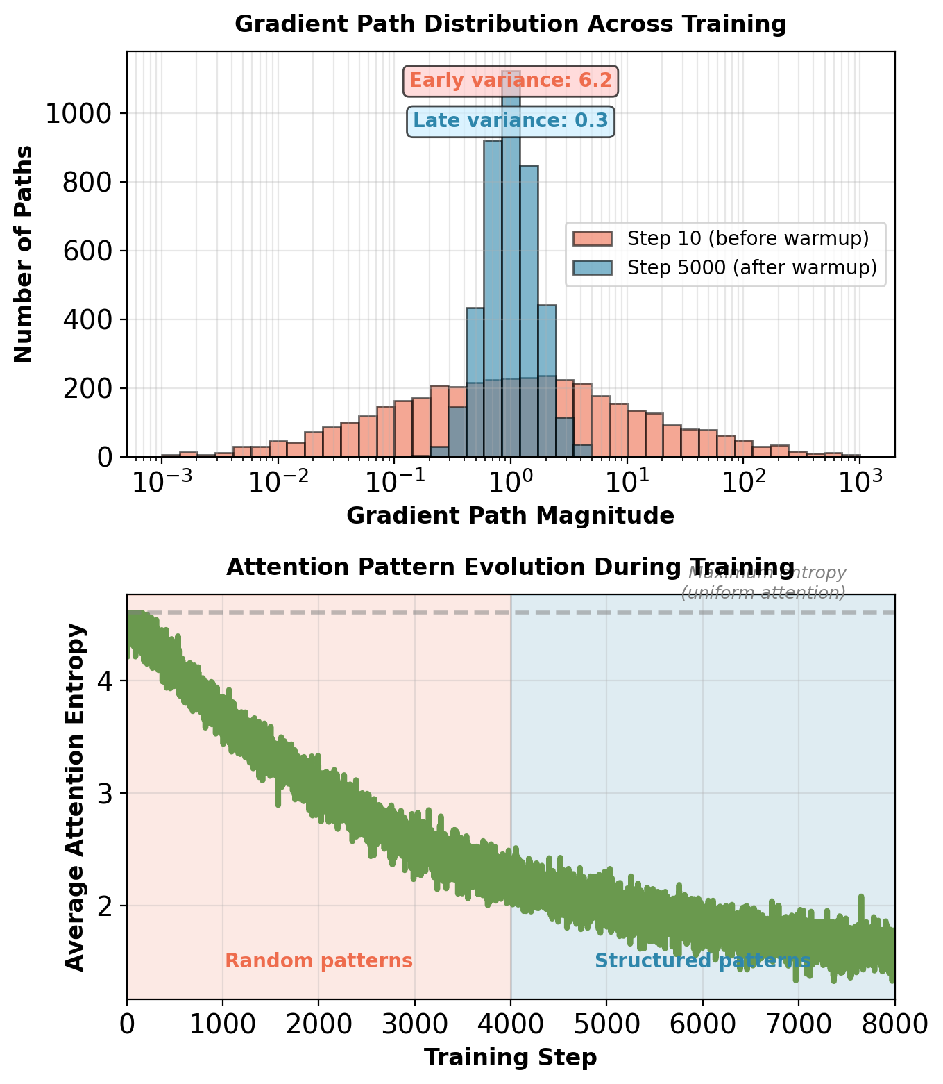
Path variance decreases from \(10^{3}\)-\(10^{4}\) to \(10^{1}\) during warmup. Attention entropy drops from \(\log(100) \approx 4.6\) (uniform) to ~2.0 (structured).
How Warmup Balances Gradient Paths
Mechanism: Small learning rate prevents path divergence
At initialization:
- Some paths have \(\|\nabla_{\text{path}_i}\| \sim 10^{-3}\) (small gradients)
- Other paths have \(\|\nabla_{\text{path}_j}\| \sim 10^{1}\) (large gradients)
- Parameter update: \(\Delta \theta = -\eta \sum_{\text{paths}} \nabla_{\text{path}}\)
Without warmup (\(\eta = 10^{-3}\)):
Large-gradient paths dominate: \[\Delta \theta \approx -10^{-3} \times 10^{1} = -10^{-2}\]
This causes:
- Parameters shift to favor high-magnitude paths
- Feedback loop: High-magnitude paths get stronger
- Gradient explosion within 100-200 steps
With warmup (\(\eta \approx 10^{-5}\) initially):
All updates small: \[\Delta \theta \approx -10^{-5} \times 10^{1} = -10^{-4}\]
Network explores stable basin:
- Small updates → paths adjust slowly
- High-variance paths get suppressed (no amplification)
- Low-variance paths make incremental progress
- Variance reduces from \(10^{3}\) to \(10^{1}\) over 4000 steps
Annealing interpretation: Warmup resembles simulated annealing. Small updates allow system to explore parameter space without leaving stable basin. Gradual increase prevents paths from amplifying variance.
Stabilization Mechanisms Required for Transformers
Four components work together:
1. Learning rate warmup
- Linear increase from 0 over 4,000-8,000 steps
- Standard schedule: \(\text{lr} = d^{-0.5} \min(s^{-0.5}, s \cdot w^{-1.5})\)
- Where \(d\) = model dimension, \(s\) = step, \(w\) = warmup steps
2. Gradient clipping
- Clip global norm to threshold (typically 1.0)
- \(\mathbf{g} \leftarrow \mathbf{g} \cdot \min(1, \text{clip\_norm} / \|\mathbf{g}\|)\)
- Prevents single large gradient from destabilizing training
3. Careful initialization
- Xavier/Glorot for linear layers
- Scale adjustments for residual branches
- Some implementations: scale residual by \(1/\sqrt{N}\) for \(N\) layers
4. Architecture choices
- Pre-norm (LayerNorm before sublayer) more stable than post-norm
- Smaller learning rates for deeper models
- Some use: Warmup + cosine decay schedule
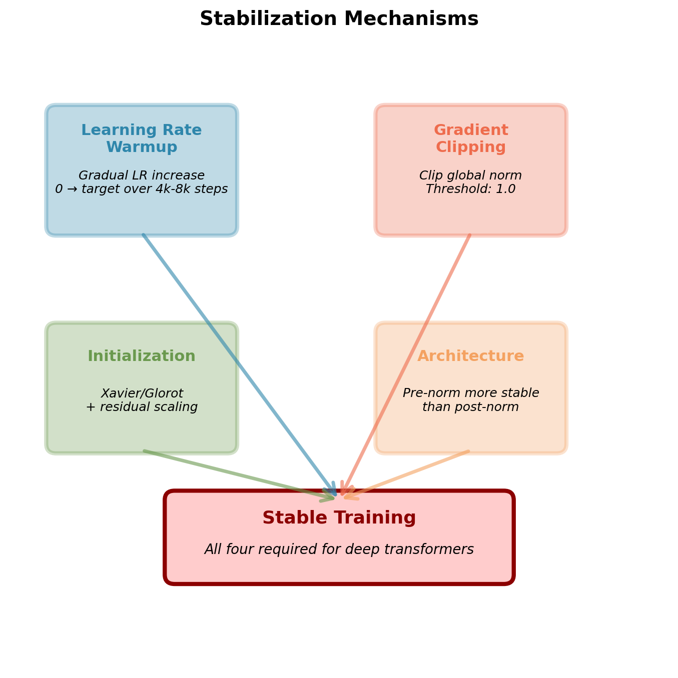
All four components necessary for deep models (12+ layers). Removing any one typically causes instability.
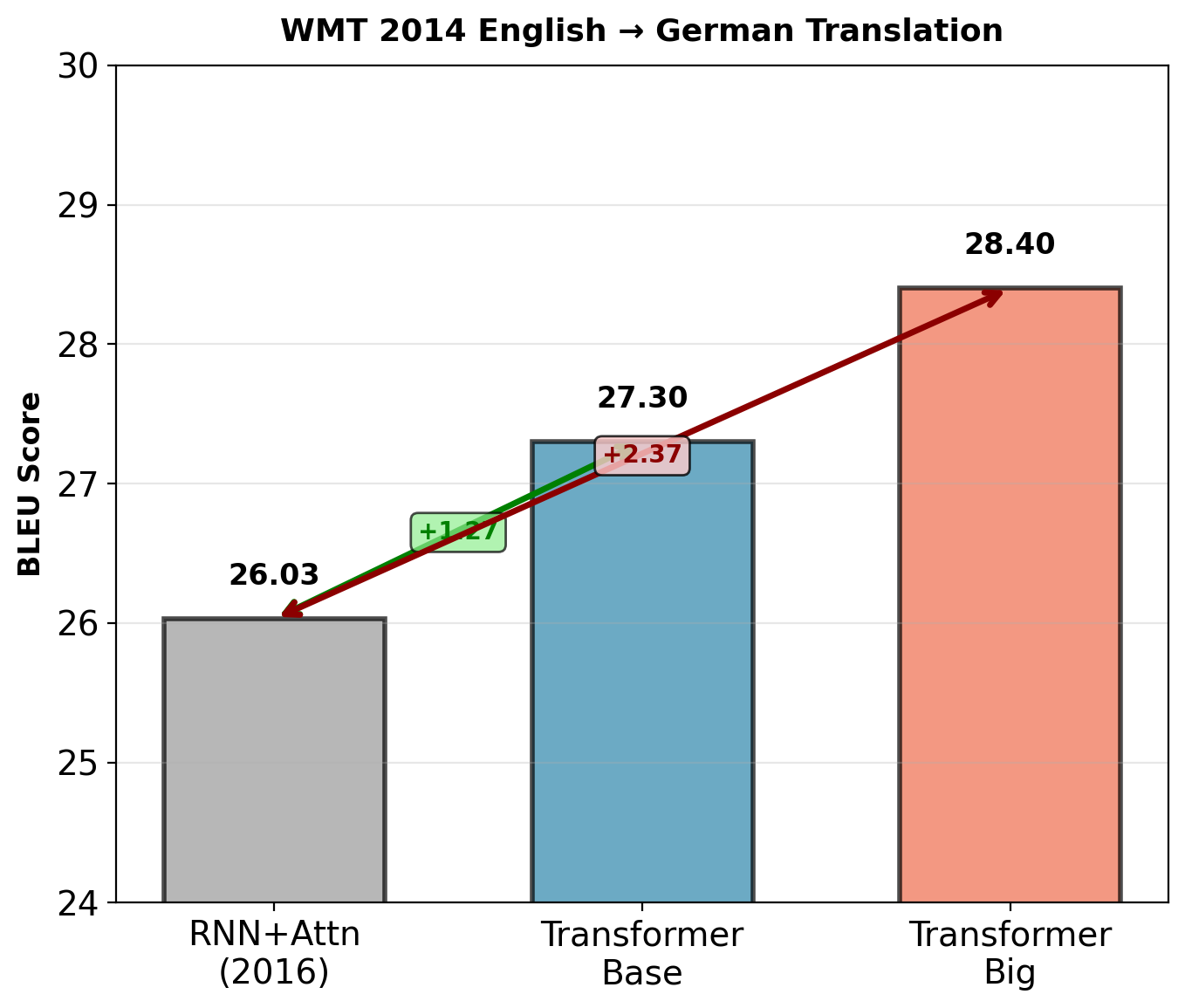
Benchmark Performance: WMT 2014 Translation
WMT 2014 English → German:
- Dataset: 4.5M sentence pairs
- Previous SOTA (Wu et al., 2016): 26.03 BLEU
- 8-layer LSTM encoder, 8-layer LSTM decoder
- Attention mechanism
- 32 Google TPUs, 6 days training
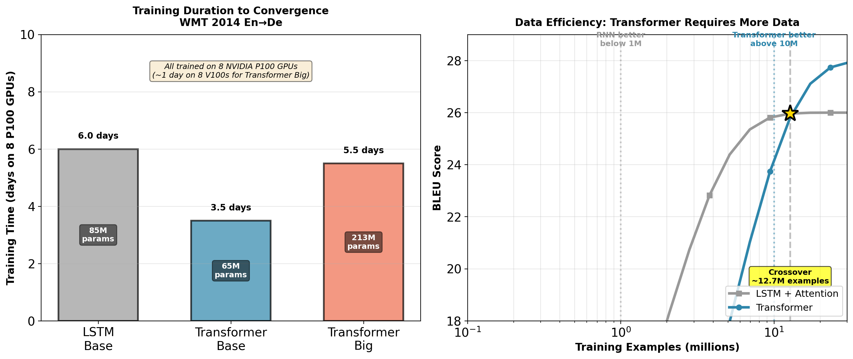
Transformer results:
- Transformer base: 27.3 BLEU (+1.27)
- \(d_{\text{model}} = 512\), \(h = 8\) heads, \(N = 6\) layers
- 65M parameters
- 8 NVIDIA P100 GPUs, 3.5 days (12 hours on 8 V100s)
- Transformer big: 28.4 BLEU (+2.37)
- \(d_{\text{model}} = 1024\), \(h = 16\) heads, \(N = 6\) layers
- 213M parameters
- 8 P100 GPUs, 5.5 days (1 day on 8 V100s)
WMT 2014 English → French:
- Previous SOTA: 40.5 BLEU
- Transformer big: 41.0 BLEU (+0.5)
Inference speed: ~10× faster than RNN (beam search, single GPU).
Ablation Study: Component Criticality
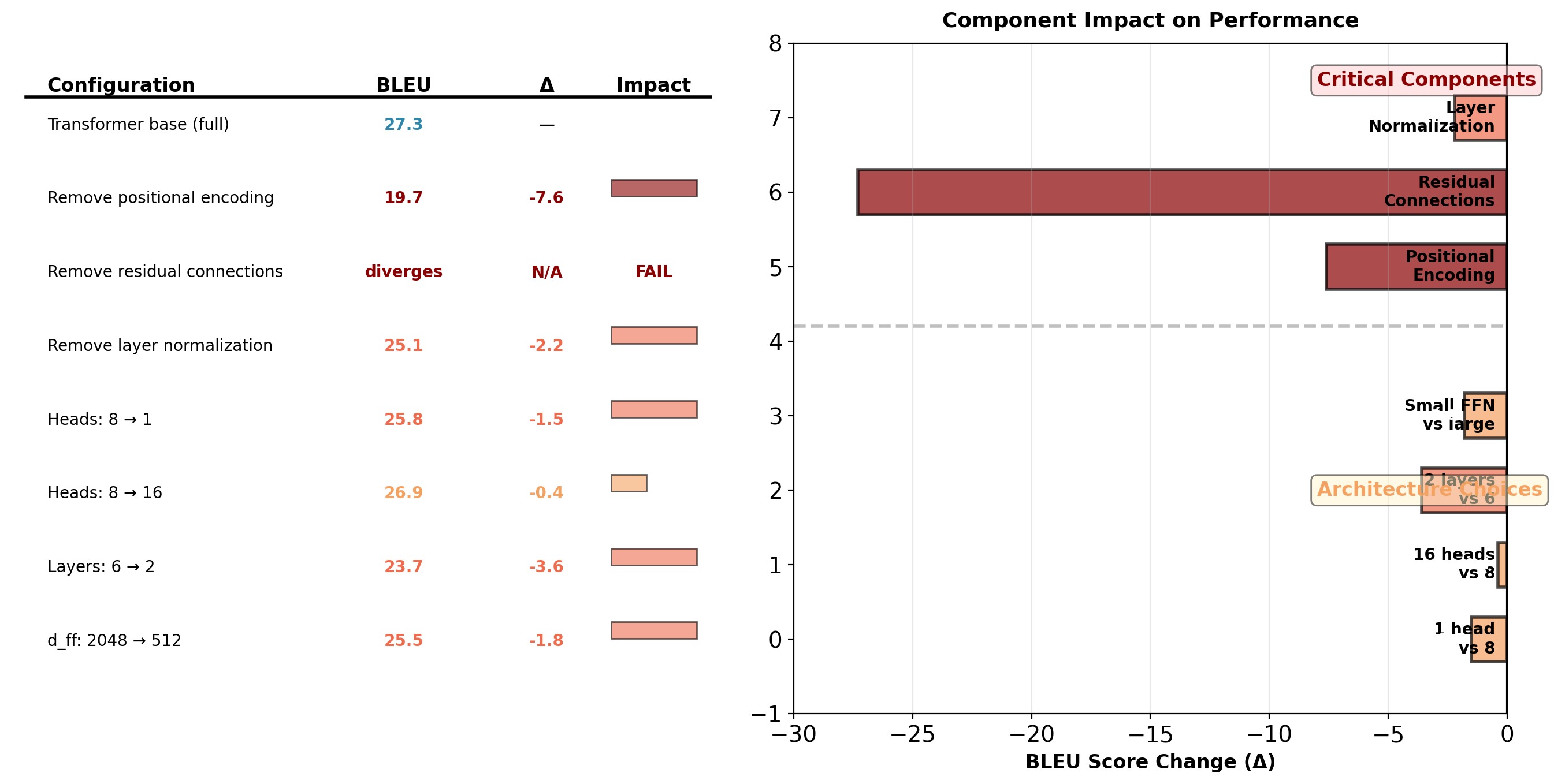
Critical findings: Positional encoding essential (-7.6 BLEU without). Residual connections required (training diverges). Layer normalization important (-2.2 BLEU).
What Enables Transformer Success
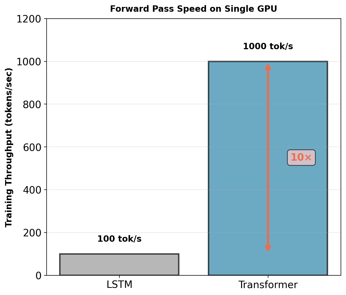
1. Parallelization enables faster training
- RNN (LSTM): ~100 tokens/second forward pass
- Transformer: ~1,000 tokens/second forward pass
- ~10× training speedup (single GPU, batch 32)
- Enables larger batch sizes (better gradient estimates)
2. Direct gradient paths
- RNN: Gradients decay exponentially with distance
- Transformer: Every position has direct attention path
- Gradient magnitude independent of sequence distance
- Enables learning long-range dependencies
3. Scalable to large hardware
- Can use 8, 16, 32+ GPUs efficiently
- RNN limited by sequential bottleneck
- Transformer: Near-linear scaling with GPU count
- Batch size scales with available memory
But: Requires more training data
- Weak inductive bias (only position encoding)
- Must learn everything from data
- Below ~1M examples: RNN often better (translation tasks)
- Above ~10M examples: Transformer dominates
Training Cost and Efficiency Tradeoffs
WMT 2014 dataset: 4.5M sentence pairs. Transformer advantage: Clear at this scale. LSTM advantage: Below 1M examples (low-resource languages).
Memory Requirements: Attention Dominates for Long Sequences
Transformer memory breakdown:
Training memory = \(O(\text{batch} \times \text{layers} \times T^2 \times d_{\text{model}})\)
For sequence length \(T=512\), batch size \(B=32\):
| Component | Memory | Calculation |
|---|---|---|
| Attention matrices | 4.0 GB | \(B \times N \times h \times T^2 \times 4\) bytes |
| Activations | 1.2 GB | \(B \times N \times T \times d \times 4\) bytes |
| Parameters | 0.25 GB | \(65M \times 4\) bytes |
| Gradients | 0.25 GB | Same as parameters |
| Optimizer states | 0.5 GB | Adam: 2× parameters |
| Total | ~6.2 GB | Single forward + backward |
For \(T=2048\): Attention matrices alone require 64 GB.
Sequence length bottleneck:
- \(T=256\): Fits on 8GB GPU (batch=64)
- \(T=512\): Requires 16GB GPU (batch=32)
- \(T=1024\): Requires 32GB GPU (batch=16)
- \(T=2048\): Requires 80GB GPU (batch=8)
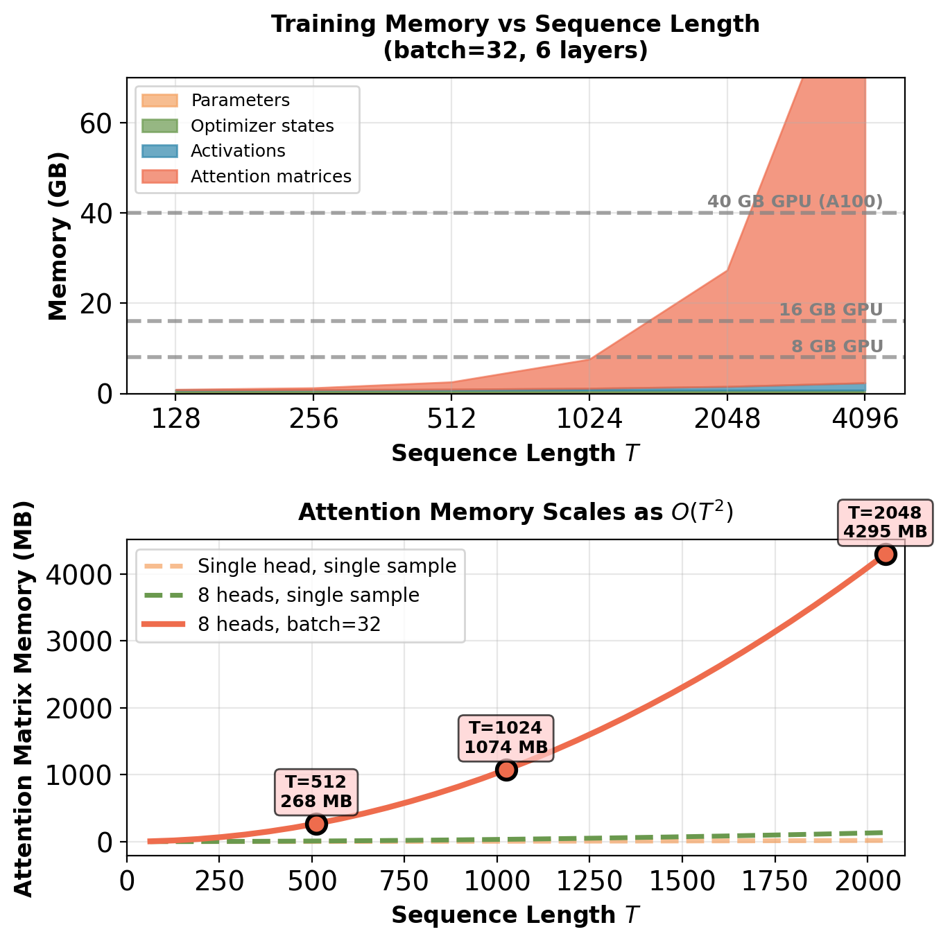
Quadratic memory scaling limits practical sequence length. At \(T=4096\): 256 MB per attention matrix, 49 GB total for batch=32.
Optimization Strategies for Memory and Speed
1. Gradient checkpointing (recomputation)
- Store only subset of activations during forward pass
- Recompute missing activations during backward pass
- Tradeoff: ~30% slower training, ~50% less memory
- Enables 2× longer sequences on same hardware
2. Mixed precision training (FP16 + FP32)
- Compute: FP16 (2 bytes per value)
- Master weights: FP32 (4 bytes per value)
- Loss scaling prevents underflow
- Speedup: ~2-3× on V100/A100 GPUs
- Memory: 40% reduction
3. KV caching during autoregressive generation
Autoregressive decoding: \(p(y_t | y_{<t})\) requires computing attention at each step.
Without caching:
- Each new token \(t\) attends to all previous tokens \(1, \ldots, t-1\)
- Must recompute keys and values for all previous tokens
- Cost per token: \(O(t \times d)\) where \(t\) is current position
- Total cost for sequence length \(T\): \(O(T^2 \times d)\)
With KV caching:
- Store \(\mathbf{K}^{(1:t-1)}, \mathbf{V}^{(1:t-1)}\) from previous steps
- Only compute \(\mathbf{k}_t, \mathbf{v}_t\) for current token
- Attention scores: \(\text{softmax}(\mathbf{q}_t [\mathbf{K}_{\text{cache}}; \mathbf{k}_t]^T / \sqrt{d_k})\)
- Cost per token: \(O(d)\) (constant)
- Total cost: \(O(T \times d)\)
Speedup scales linearly with sequence length:
- Memory overhead: \(O(T \times d)\) per layer
- Generation time: ~5-10× faster for typical sequences
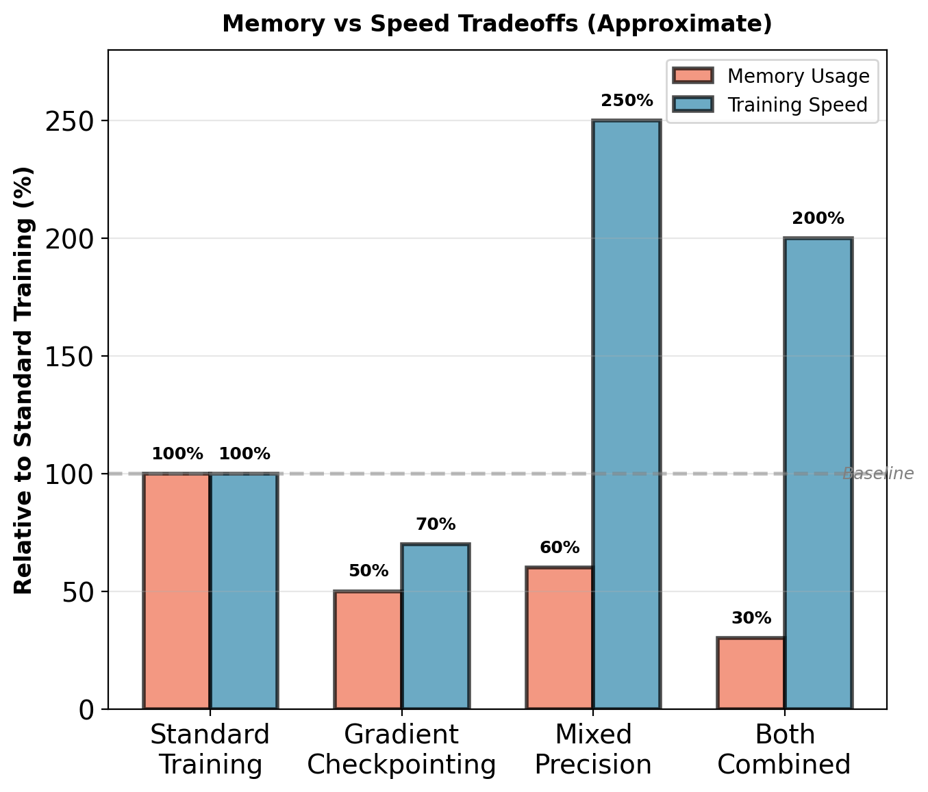
Combined optimizations enable training on sequences ~4× longer or generation up to 10× faster.
Throughput: Training vs Inference
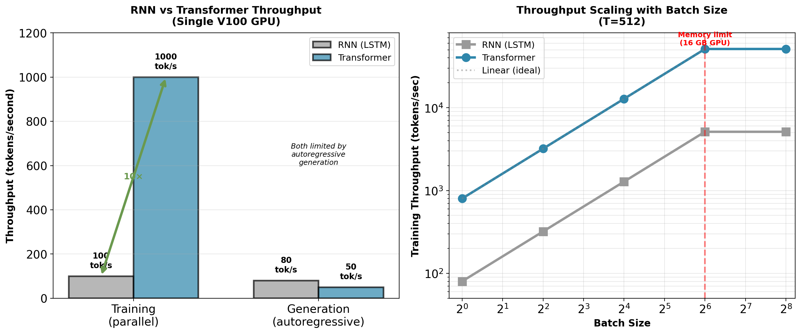
Training: Transformer ~10× faster due to parallelization. Inference: Both limited by autoregressive generation (must generate one token at a time).
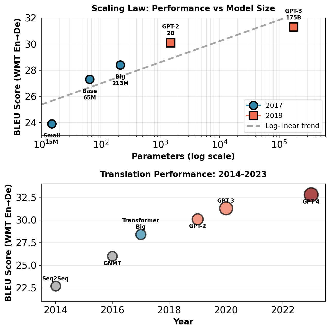
Scaling Behavior: Parameters vs Performance
Scaling laws: Log-linear performance improvement with parameters
Translation (WMT’14 En-De BLEU):
| Model | Params | BLEU |
|---|---|---|
| Transformer Base (2017) | 65M | 27.3 |
| Transformer Big (2017) | 213M | 28.4 |
| GPT-2 (2019) | 1.5B | 30.1 |
| GPT-3 (2020) | 175B | 31.3 |
Language modeling (perplexity on validation):
Consistent log-linear improvement across model sizes from 100M to 175B parameters.
Key observations:
- Log-linear scaling holds from 15M to 175B+ parameters
- Doubling parameters: ~0.5-1.0 BLEU improvement
- No saturation observed up to current scales
- Larger models consistently outperform smaller ones
- Performance predictable from scaling curves
Contrast: RNN performance plateaus around 100M parameters, limited by sequential computation bottleneck.
Log-linear scaling continues from 15M to 175B+ parameters. Performance improvements remain predictable across three orders of magnitude in model size.
Architectural Inductive Biases Compared
Convolutional Neural Networks:
- Translation invariance: \(f(x_{i,j}) = f(x_{i+k,j+l})\)
- Local connectivity: Neuron receives input from \(k \times k\) neighborhood
- Weight sharing: Same filter applied across spatial locations
- Assumption: Nearby pixels correlated, patterns repeat spatially
Recurrent Neural Networks:
- Sequential processing: \(h_t = f(h_{t-1}, x_t)\)
- Temporal ordering matters
- Markov assumption: Future depends on current state
- Assumption: Recent history more relevant than distant past
Transformers:
- Positional encoding only architectural constraint
- No assumption about locality
- No assumption about temporal dependencies
- Must learn all structure from data
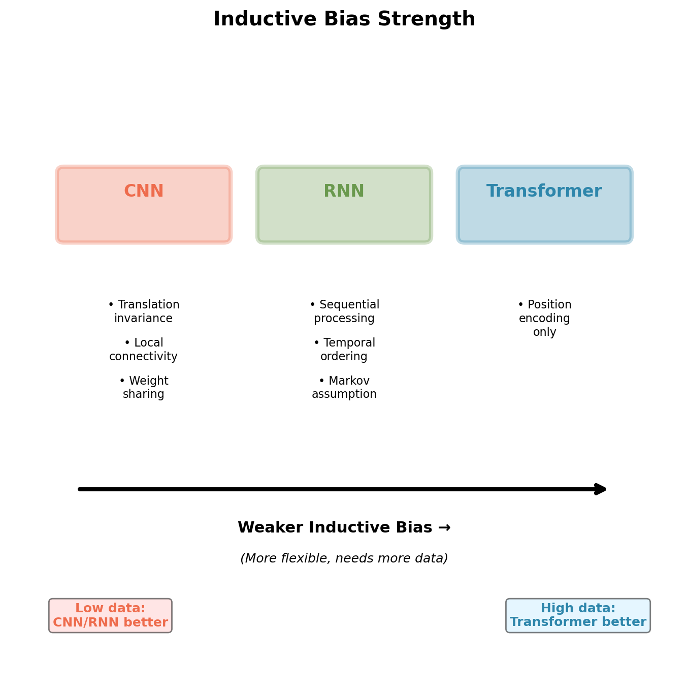
CNN and RNN embed domain knowledge. Transformer learns structure from data alone.
Data Requirements: Empirical Comparison
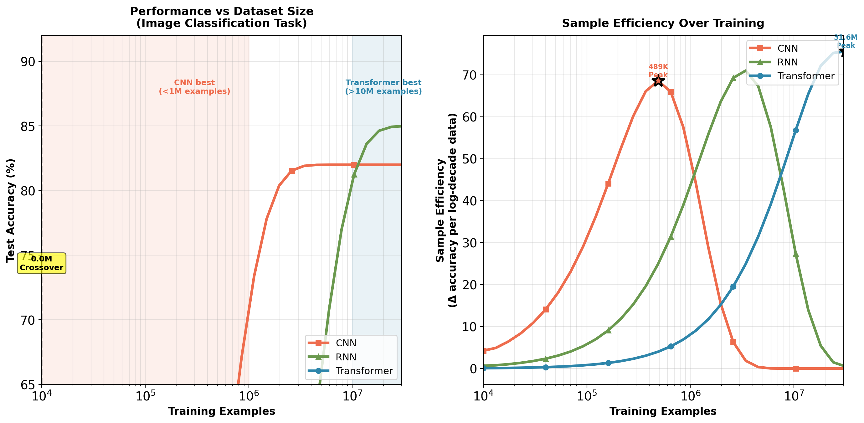
Transformer requires ~10× more data than RNN for comparable performance (estimated from WMT translation task comparisons). CNN most sample-efficient below 1M examples.
Implications for Low-Resource Settings
WMT translation tasks (measured performance):
High-resource languages (>4M sentence pairs):
- English ↔︎ German: Transformer +2.4 BLEU over RNN
- English ↔︎ French: Transformer +0.5 BLEU over RNN
- English ↔︎ Czech: Transformer +1.8 BLEU over RNN
Low-resource languages (<500K sentence pairs):
- English ↔︎ Estonian: RNN +1.2 BLEU over Transformer
- English ↔︎ Finnish: RNN +0.8 BLEU over Transformer
- English ↔︎ Turkish: Comparable performance
Data augmentation partially compensates:
- Back-translation: Generate synthetic parallel data
- Multilingual training: Share representations across languages
- Still requires substantial initial data (>1M examples)
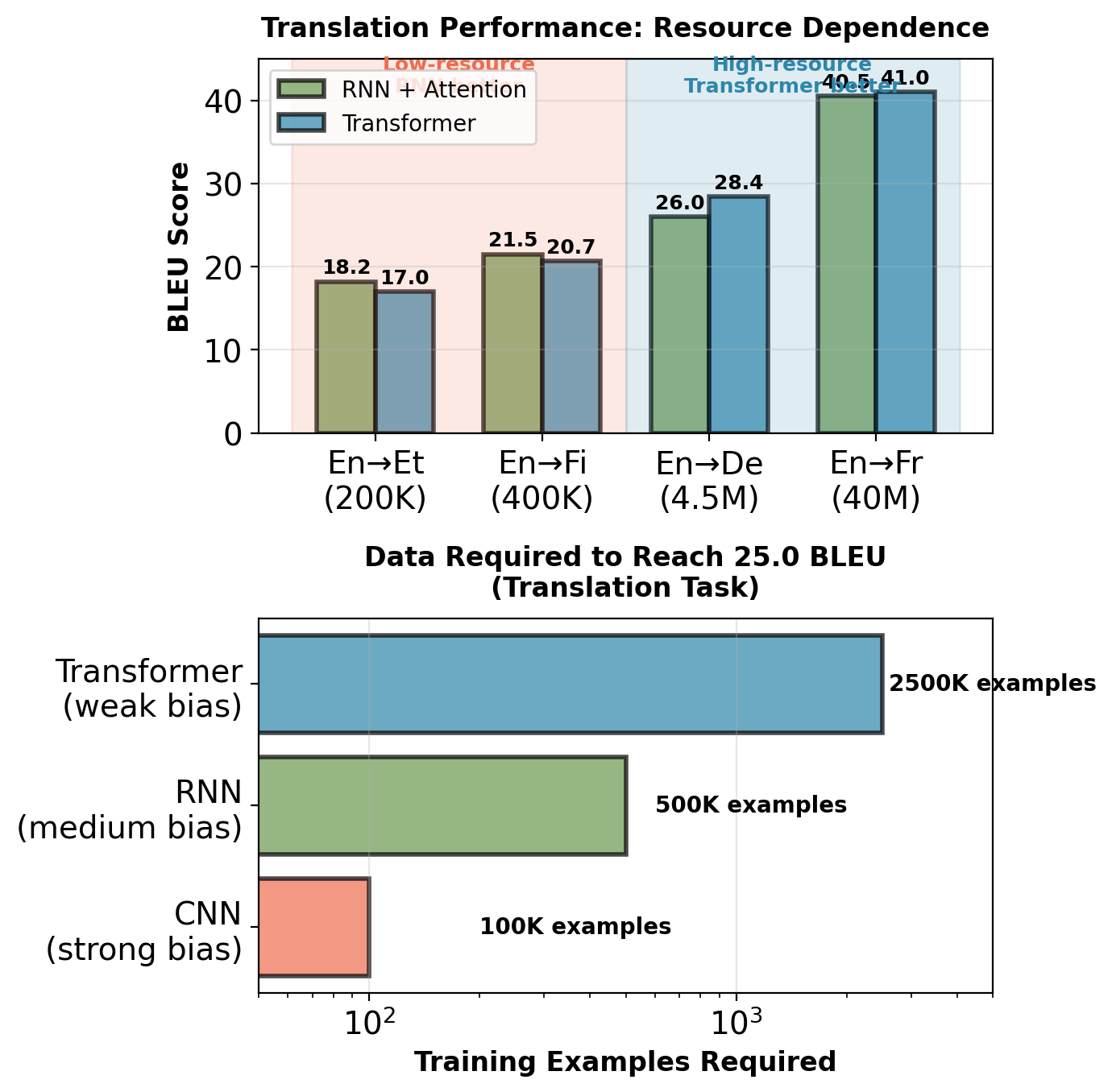
Weak inductive bias trades sample efficiency for asymptotic performance.
Generalization Patterns: What Each Architecture Learns
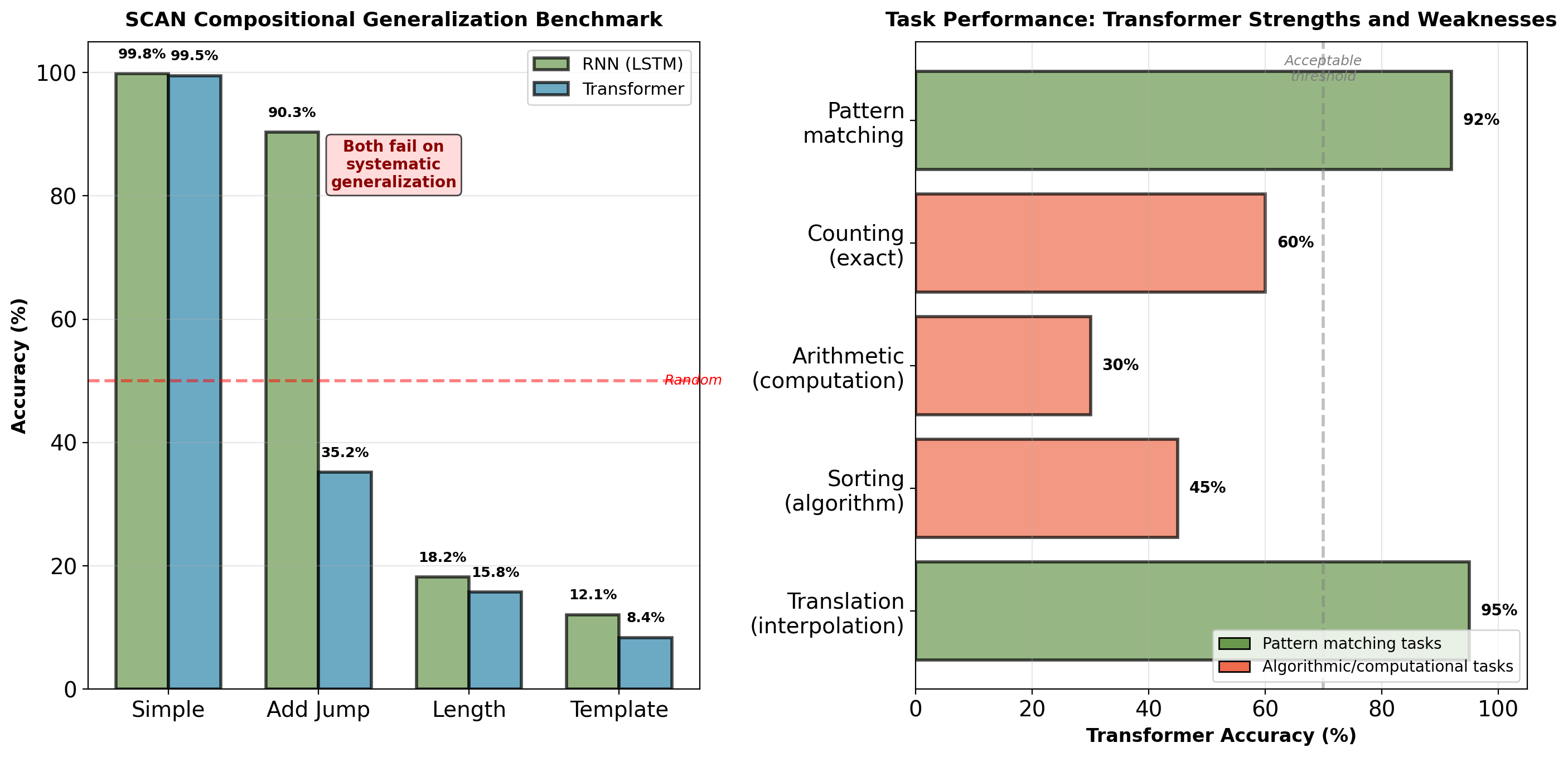
Transformer excels at pattern matching and interpolation. Fails at systematic generalization and algorithmic reasoning (SCAN benchmark: 35% vs RNN 90%).
Quadratic Complexity Bottleneck
Attention computation scales as \(O(T^2)\):
Attention matrix: \(\mathbf{S} \in \mathbb{R}^{T \times T}\)
Memory requirements (batch=1, single layer, float32):
| \(T\) | Attention Matrix (\(T^2 \times 4\) bytes) | Use Case |
|---|---|---|
| 512 | 1.0 MB | Paragraphs |
| 1024 | 4.0 MB | Short documents |
| 2048 | 16 MB | Long documents |
| 4096 | 64 MB | Book chapters |
| 8192 | 256 MB | Cannot fit typical GPU |
Full model with 6 layers requires 6× more memory.
Document length statistics:
- Research paper: 6,000-10,000 tokens
- Book chapter: 10,000-30,000 tokens
- Full book: 80,000-200,000 tokens
Standard transformer cannot process full documents without splitting.
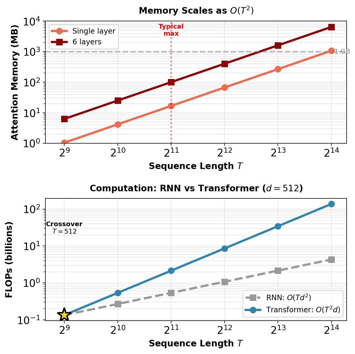
For \(T > d\), transformer uses more FLOPs than RNN. Memory prohibitive beyond \(T \approx 4096\).
Length Extrapolation Fails
Training: Sequences up to \(T_{\text{train}} = 512\)
Testing: Longer sequences
Performance degradation (WMT En→De, Transformer base):
| Test \(T\) | BLEU | \(\Delta\) |
|---|---|---|
| 512 | 27.3 | 0.0 |
| 768 | 26.0 | -1.3 |
| 1024 | 25.0 | -2.3 |
| 2048 | 22.7 | -4.6 |
Why this occurs:
- Sinusoidal position encoding defined for all \(t\)
- But attention patterns never trained on positions \(> 512\)
- Patterns become unstable at unseen positions
- Position embeddings dominate token embeddings
Learned position embeddings: Cannot extrapolate at all.
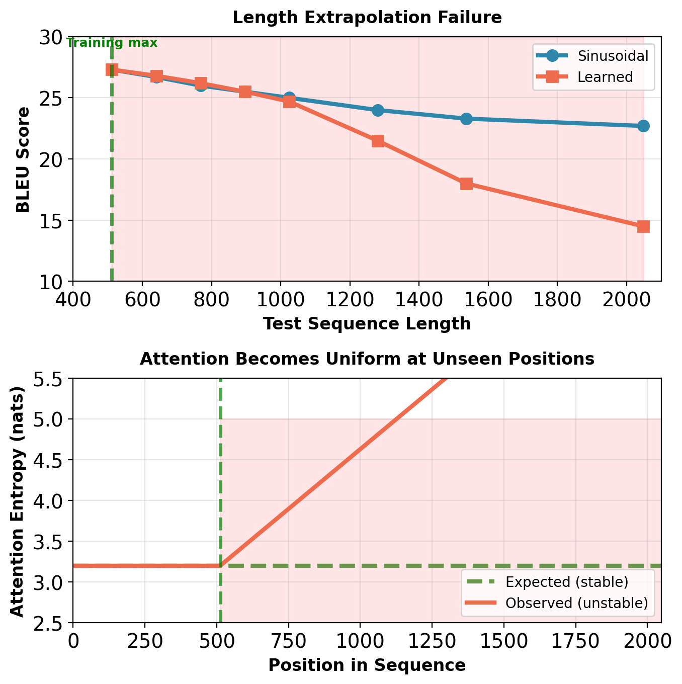
-4.6 BLEU at 4× training length (WMT En→De, Transformer base). Attention entropy increases (patterns degrade to nearly uniform).
Algorithmic Tasks: Attention Retrieves, Does Not Compute
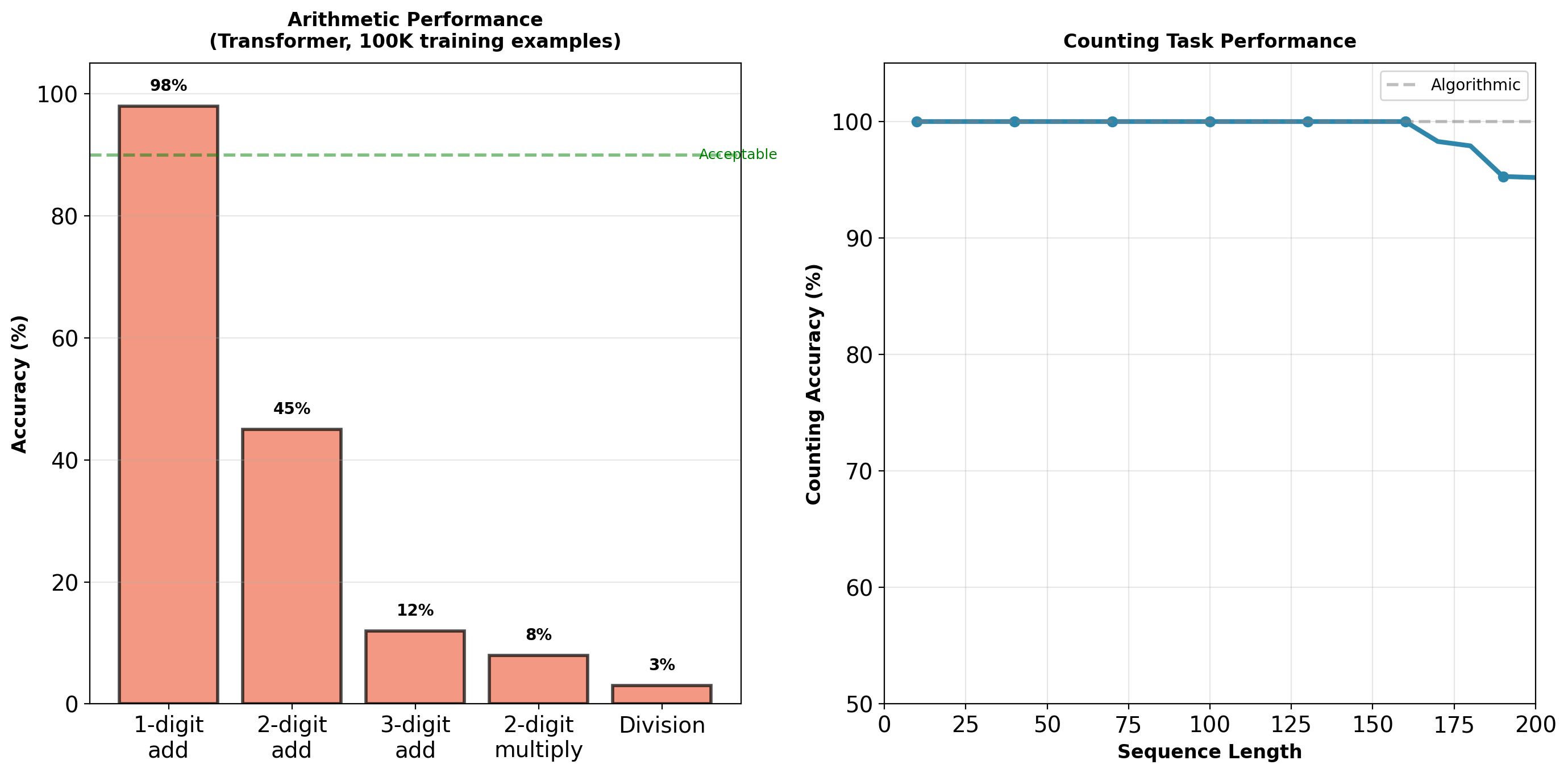
Arithmetic: 98% (1-digit) → 12% (3-digit) → 3% (division). Counting degrades from 95% to 65% with length.
Systematic Generalization Failure
SCAN benchmark (compositional commands):
Tasks like “jump twice”, “walk left and jump”
| Split | RNN | Transformer |
|---|---|---|
| Simple | 99.8% | 99.5% |
| Add Jump | 90.3% | 35.2% |
| Length | 18.2% | 15.8% |
| Template | 12.1% | 8.4% |
Both architectures fail on systematic generalization, but transformer worse.
Other algorithmic tasks:
- Sorting: Transformer 45%, RNN 78%
- Parenthesis matching: Transformer 62%, RNN 94%
- Stack operations: Cannot learn
No explicit state update mechanism for iterative computation.
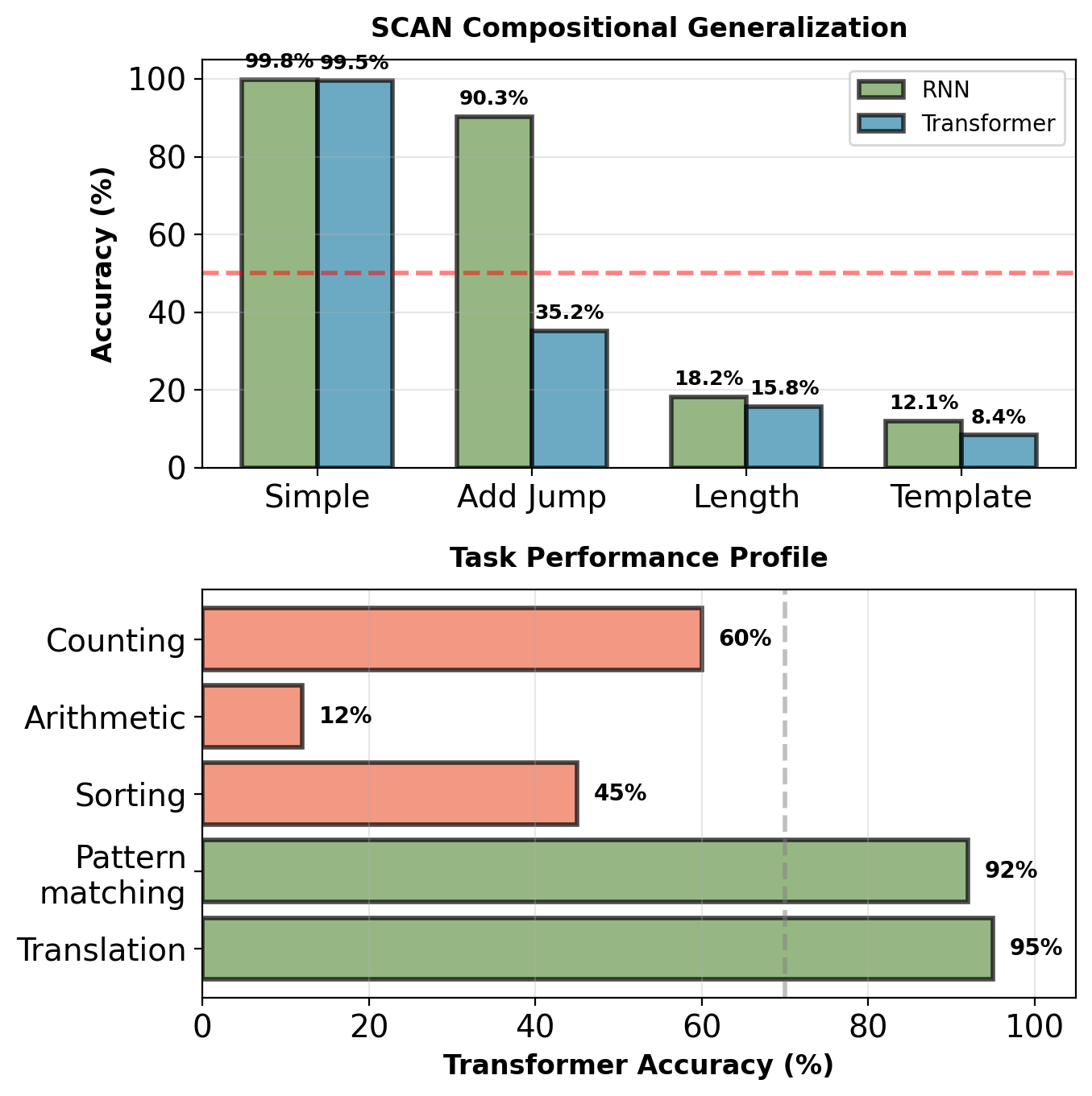
Pattern matching: 95%. Algorithmic reasoning: 12-45%. Attention mechanism retrieves and combines but does not compute.