Modern Large Language Models
EE 641 - Unit 7
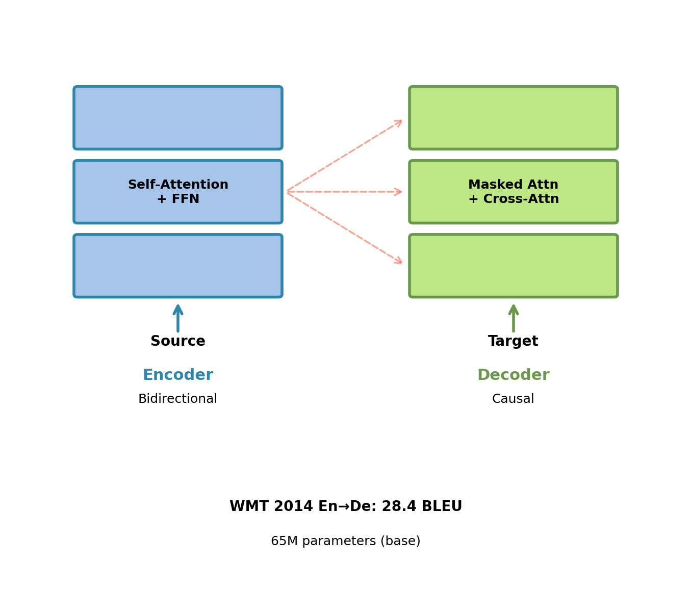
Attention Patterns Determine Information Flow
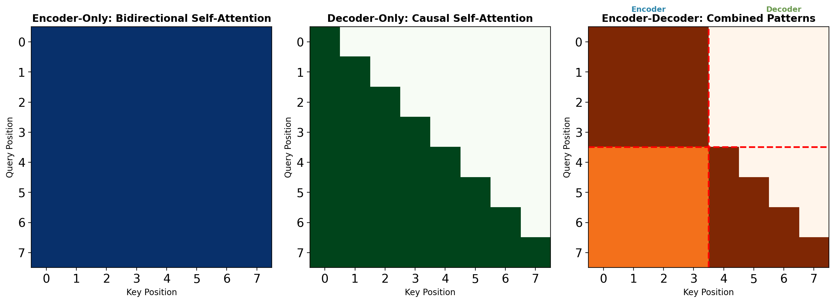
White = attention allowed (value 1.0), Dark = masked (value 0)
Encoder-only: All positions attend to all positions simultaneously.
Decoder-only: Position \(i\) attends only to positions \(j \leq i\) (lower triangular).
Encoder-decoder: Encoder positions bidirectional, decoder positions causal with cross-attention.
Language Modeling: Every Token as Supervision
Supervised classification requires annotation:
Example: Sentiment classification
Input:  "This movie was excellent"
Label:  positive    # Human annotator needed
Annotation costs:
- $0.10 - $1.00 per example
- Quality control adds 30-50% overhead
- Domain expertise increases cost 5-10×
Scale limitations:
- ImageNet: 1.4M images, $1M+ cost
- SQuAD v2: 150K examples, ~$150K cost
- GLUE (all tasks): 400K examples total
Language modeling uses text structure:
Example: Next token prediction
Input:  ["The", "cat", "sat", "on"]
Target: ["cat", "sat", "on", "the"]
No annotation needed:
- Supervision derived from token sequence
- Every position provides training signal
- Cost: $0 per example
- Only requirement: Clean text
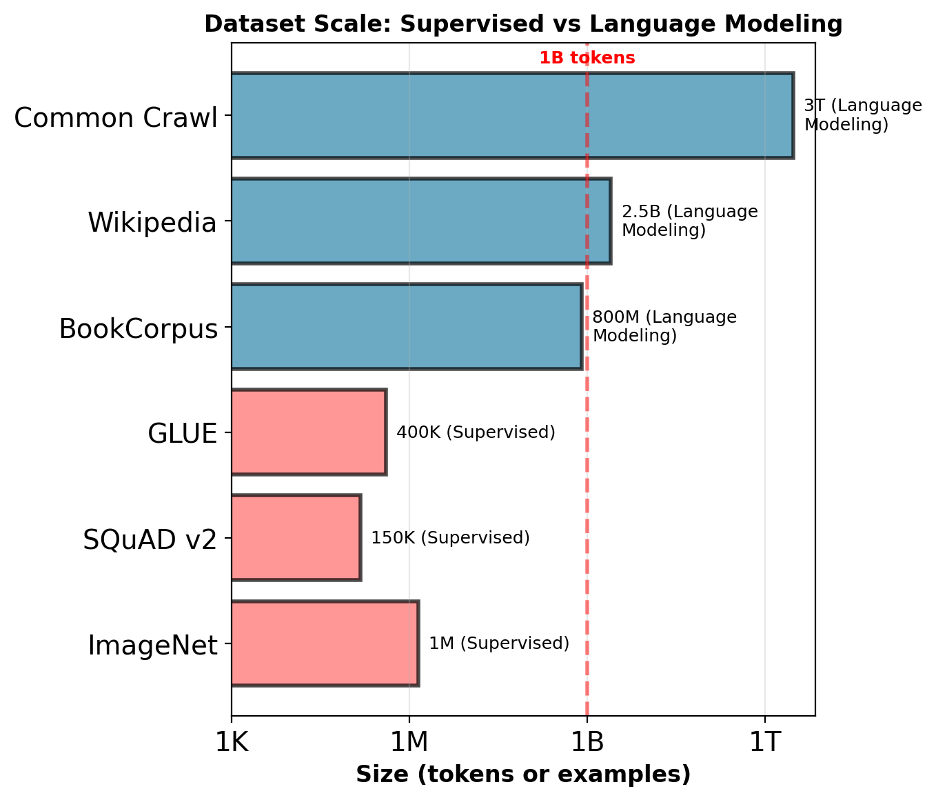
Common Crawl: 3 trillion tokens. 10,000× larger than largest supervised dataset.
Language modeling converts unlimited unlabeled text into training data.
Loss Scales as Power Law in Parameters
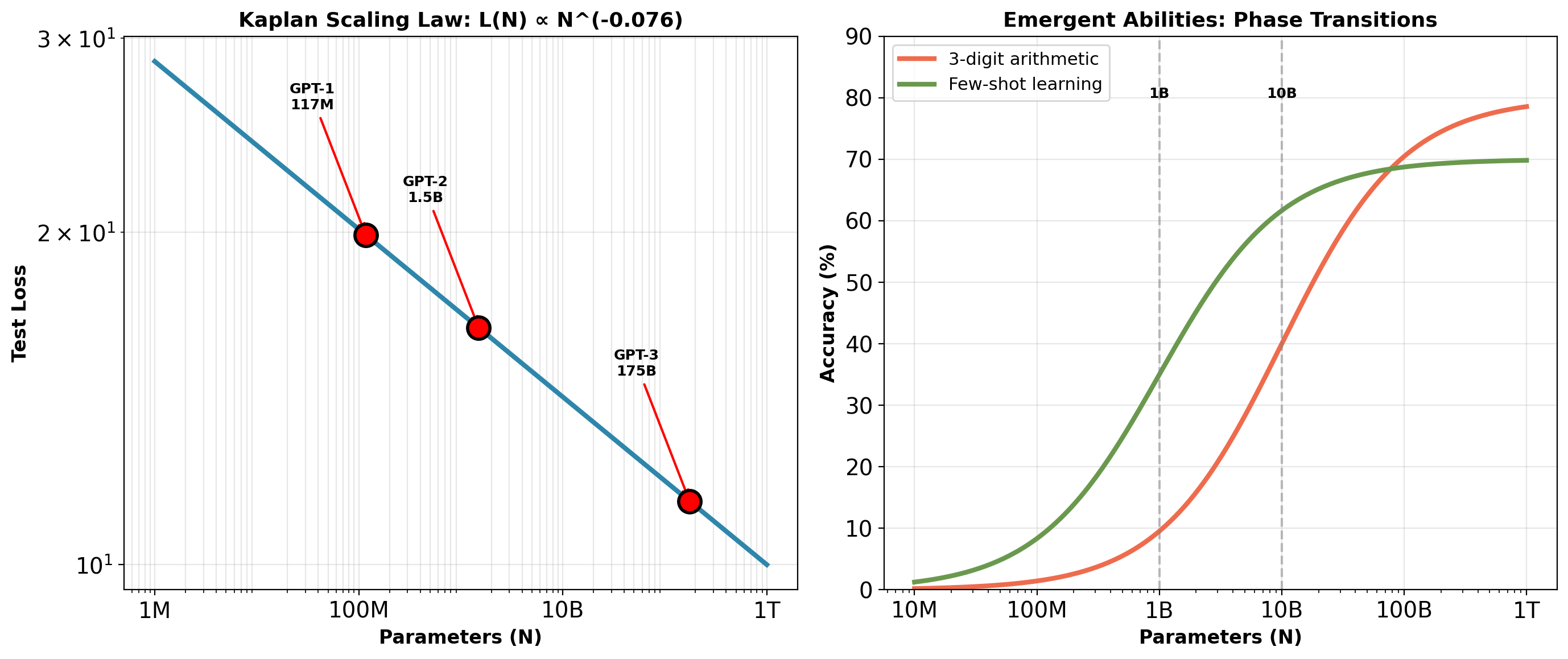
Left: Test loss decreases smoothly as power law in parameters (Kaplan et al., 2020)
Right: Task accuracy shows step-function behavior at specific parameter thresholds
Performance becomes predictable. Emergence remains surprising.
From Transformer to BERT: Encoder-Only Design
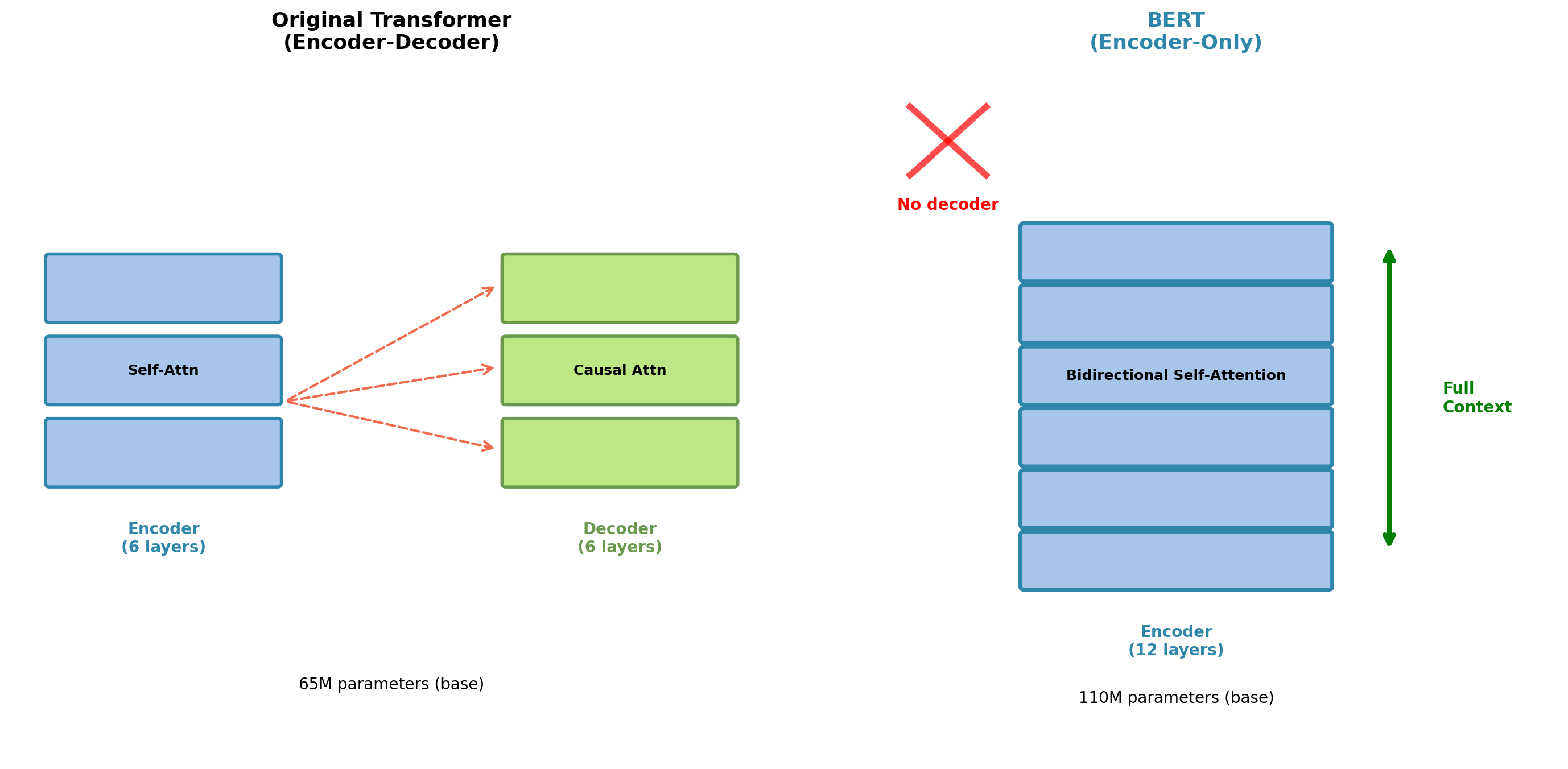
Architectural modifications:
Remove decoder stack and cross-attention entirely.
Increase encoder depth: 6 → 12 layers
Increase width: H = 512 → 768
| Component | Transformer | BERT-base |
|---|---|---|
| Encoder layers | 6 | 12 |
| Decoder layers | 6 | 0 |
| Hidden size (H) | 512 | 768 |
| Attention heads | 8 | 12 |
| Parameters | 65M | 110M |
Design choices:
Head dimension fixed at 64 across all configs (empirically optimal).
FFN expansion ratio 4×: \(d_{\text{ff}} = 4H = 3072\)
Depth over width: 12×768 outperforms 6×1088 (80.5 vs 78.1 GLUE, same FLOPs)
All layers use bidirectional self-attention (no causal masking).
Bidirectional Self-Attention
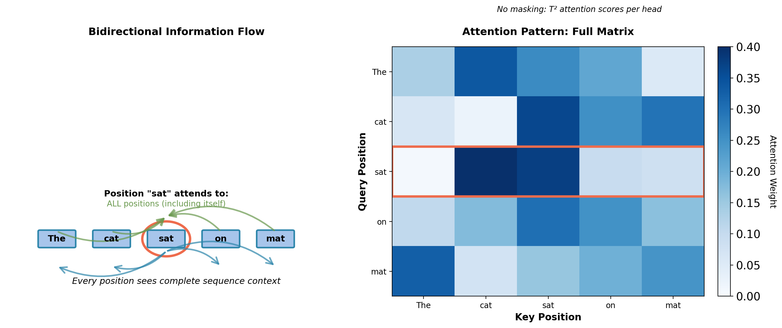
Attention complexity: Each layer computes \(O(T^2 d)\) operations.
For T=512, H=768, A=12 heads: Self-attention performs 403M multiply-adds per layer (Q/K/V projections: 906M, attention scores + output: 403M).
FFN performs 2.4B multiply-adds (two 768→3072→768 projections).
Per layer total: ~2.2B FLOPs. 12 layers: ~27B FLOPs per sequence.
Input Embeddings: Three Learned Representations
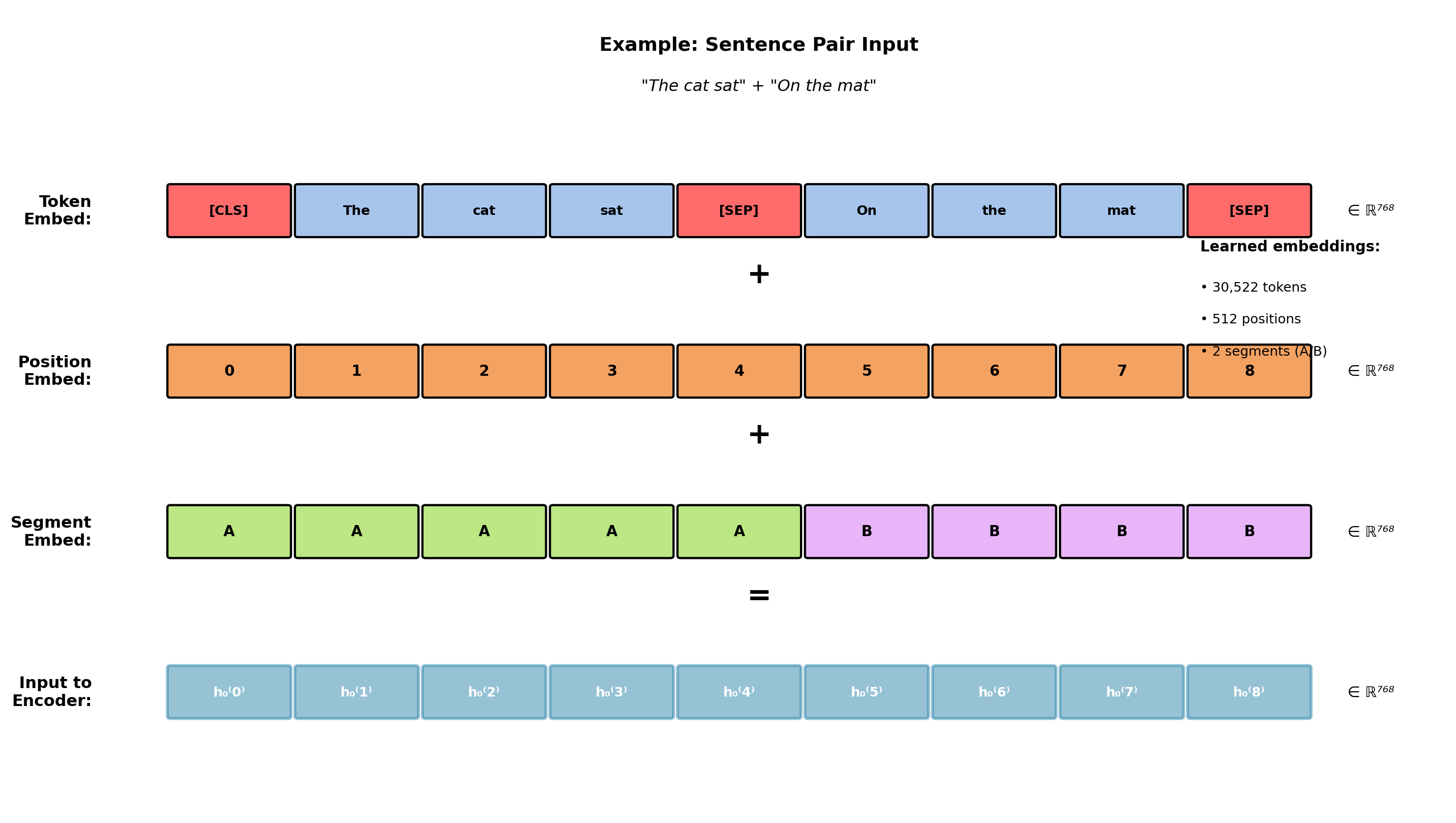
\[\mathbf{h}_0^{(i)} = \mathbf{E}_{\text{token}}[x_i] + \mathbf{E}_{\text{position}}[i] + \mathbf{E}_{\text{segment}}[s_i]\]
Token embeddings: WordPiece vocabulary of 30,522 subwords. Matrix \(\mathbf{E}_{\text{token}} \in \mathbb{R}^{30522 \times 768}\) contains 23.4M parameters (21% of model).
Position embeddings: Learned (not sinusoidal). Matrix \(\mathbf{E}_{\text{position}} \in \mathbb{R}^{512 \times 768}\) for max length 512. Ablation: learned positions outperform sinusoidal by +0.7 GLUE points.
Segment embeddings: Binary A/B indicator. Matrix \(\mathbf{E}_{\text{segment}} \in \mathbb{R}^{2 \times 768}\) distinguishes sentence pairs for pre-training (Next Sentence Prediction) and fine-tuning tasks (QA, entailment).
[CLS] Token Aggregates Sequence Information
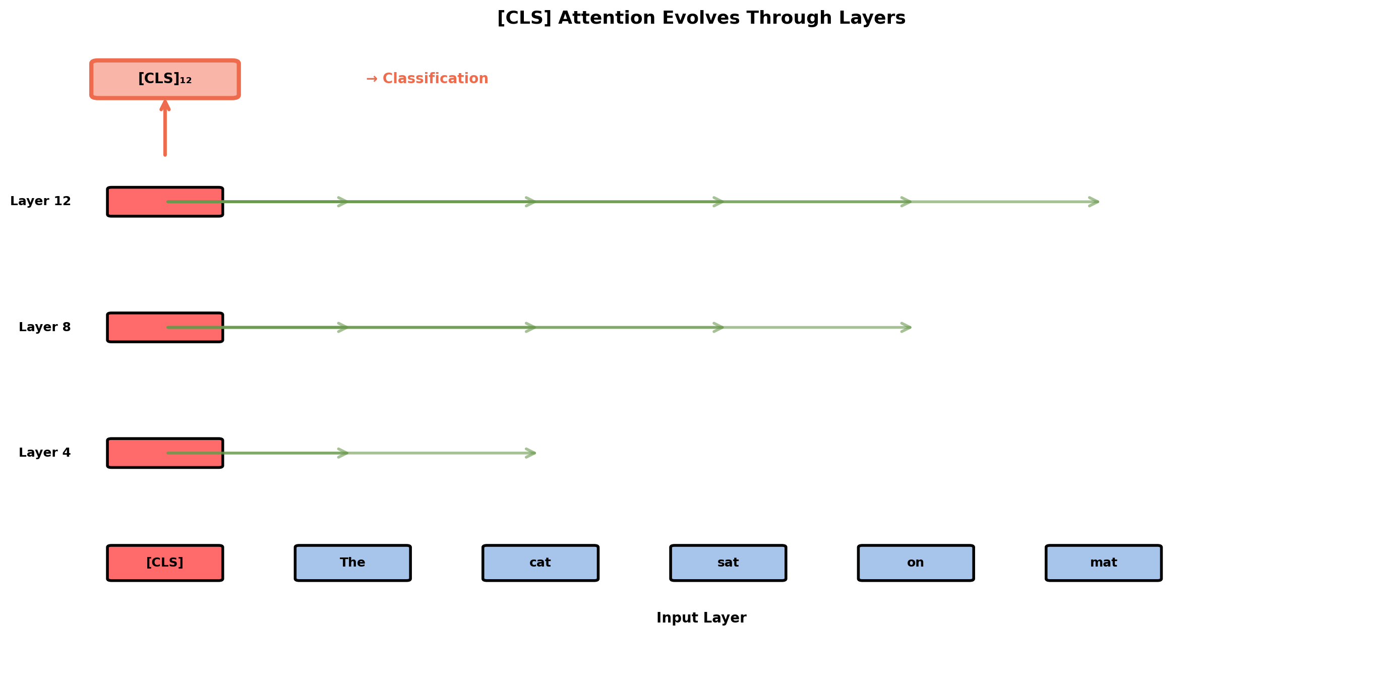
Classification mechanism:
Final [CLS] representation \(\mathbf{h}_{\text{[CLS]}}^{(12)} \in \mathbb{R}^{768}\) passed to task head:
\[\mathbf{z} = \mathbf{W}\mathbf{h}_{\text{[CLS]}}^{(12)} + \mathbf{b}\]
where \(\mathbf{W} \in \mathbb{R}^{K \times 768}\) for K classes.
Why [CLS] outperforms pooling:
| Method | MNLI | QQP | SST-2 | Avg |
|---|---|---|---|---|
| [CLS] token | 84.6% | 89.2% | 93.5% | 89.1% |
| Mean pooling | 83.9% | 88.4% | 92.7% | 88.3% |
| Max pooling | 83.2% | 87.9% | 92.1% | 87.7% |
+0.8 to +1.4 points improvement.
Learned vs fixed aggregation:
[CLS] learns task-specific attention during fine-tuning.
Analysis (Clark et al., 2019) of [CLS] attention in layers 11-12:
- Sentiment tasks: Focuses on adjectives (avg weight 0.45)
- NER: Distributes broadly (avg weight 0.12 per token)
- QA: Focuses on question words (avg weight 0.38)
Mean pooling assigns fixed 1/T weight per token. Cannot adapt to task structure.
Hierarchical Representations: Layer-by-Layer Specialization
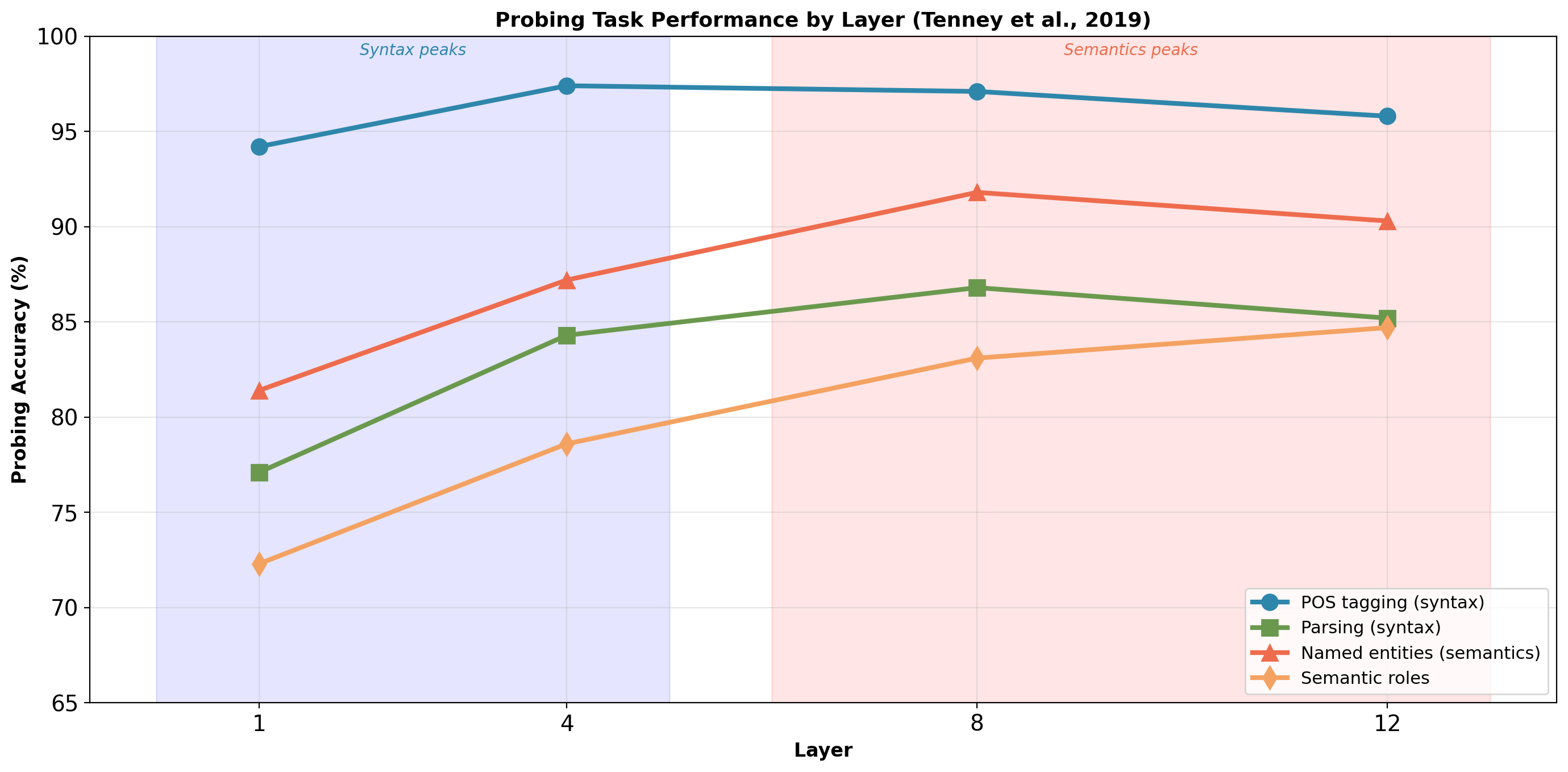
Probing methodology (Tenney et al., 2019): Train linear classifiers on frozen BERT representations at each layer.
Pattern: Syntax peaks early (POS at layer 4: 97.4%), semantics peaks mid-network (NER at layer 8: 91.8%), task-specific features emerge late (semantic roles at layer 12: 84.7%).
Transfer learning implication: Fine-tuning updates upper layers more aggressively (2× learning rate for layers 7-12, 5× for classification head). Lower layers provide general linguistic features.
Computational Profile: Memory-Bound Operation
Per-layer computation (T=512, H=768):
| Component | FLOPs | % |
|---|---|---|
| Q/K/V projections | 906M | 40% |
| Attention scores + output | 403M | 18% |
| Output projection | 302M | 13% |
| FFN (2 layers) | 2,414M | 107% |
| Per layer total | ~2.2B | |
| 12 layers | ~27B |
FFN dominates compute (2.4B vs 1.6B for all attention operations).
Memory bandwidth bottleneck:
V100: 125 TFLOPS peak, 900 GB/s bandwidth
Model size: 440 MB (110M params × 4 bytes)
Arithmetic intensity (batch=1): 27B / 440MB = 61 FLOPs/byte
Required for compute-bound: 125 TFLOPS / 900 GB/s = 139 FLOPs/byte
BERT is memory-bound by 2.3×. Bottleneck is loading parameters from HBM, not compute.
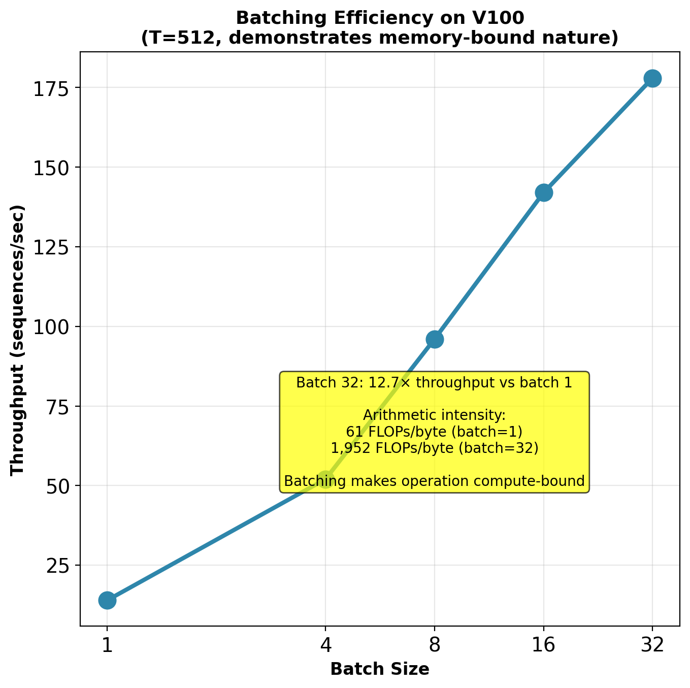
At batch=1: theoretical time (compute-bound) = 0.22 ms, actual = 70 ms (318× slower due to memory bandwidth).
At batch=32: parameters loaded once, used 32× → compute-bound regime (14× slower vs 318×).
The Bidirectional Training Problem
Standard language modeling objective requires causal masking:
\[\mathcal{L}_{\text{LM}} = -\sum_{i=1}^{T} \log P(x_i | x_{<i}; \theta)\]
Position \(i\) predicts from only \(x_1, \ldots, x_{i-1}\). Cannot see \(x_{i+1}, \ldots, x_T\).
BERT architecture is bidirectional. Position \(i\) attends to all positions through self-attention.
If we apply standard LM with bidirectional attention:
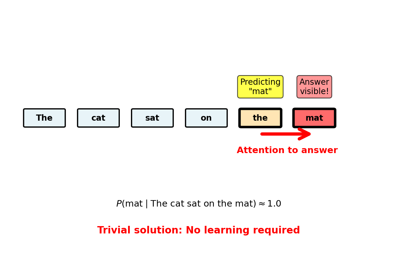
Consider predicting “mat” from context:
The cat sat on the ___With bidirectional attention: - Model attends to: “The”, “cat”, “sat”, “on”, “the” - Also attends to: “mat” (the answer!)
Through attention weights, model copies answer from future context.
Empirical verification (Devlin et al., 2018): - Bidirectional model on standard LM: Train loss → 0 instantly - Test loss: Explodes on any input perturbation - Model memorizes position-specific shortcuts, learns nothing
This trivial solution prevents any learning of linguistic structure.
Need objective that uses bidirectional context without revealing answers.
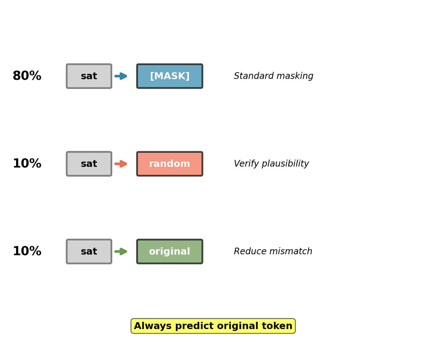
Masking Strategy: 80% / 10% / 10% Split
For each token selected in \(\mathcal{M}\), corrupt with probability distribution:
\[\tilde{x}_i = \begin{cases} \texttt{[MASK]} & \text{with probability } 0.8 \\ x_j \sim \text{Uniform}(\mathcal{V} \backslash \{x_i\}) & \text{with probability } 0.1 \\ x_i & \text{with probability } 0.1 \end{cases}\]
where \(\mathcal{V}\) is vocabulary.
Case 1: Replace with [MASK] (80%)
Original: The cat sat on the mat
Corrupt:  The cat [MASK] on the mat
Predict:  sat
Standard masked prediction. Model learns from context.
Case 2: Replace with random token (10%)
Original: The cat sat on the mat
Corrupt:  The cat dog on the mat
Predict:  sat (not dog!)
Forces model to verify plausibility from context. Cannot trust observed token.
Prevents model learning: “token is wrong → predict based on syntax only”
Model must use semantics: “dog” is implausible subject for “on mat” → predict “sat”
Case 3: Keep original token (10%)
Original: The cat sat on the mat
Corrupt:  The cat sat on the mat
Predict:  sat
Reduces train-test mismatch. [MASK] token absent during fine-tuning.
Model learns representations useful for original tokens, not just [MASK].
Why not 100% [MASK]?
Ablation (Devlin et al., 2018): - 100% [MASK]: 78.9 GLUE score - 80/10/10 split: 80.5 GLUE score - Improvement: +1.6 points
Random token replacement prevents over-fitting to [MASK] token patterns.
MLM Training Dynamics
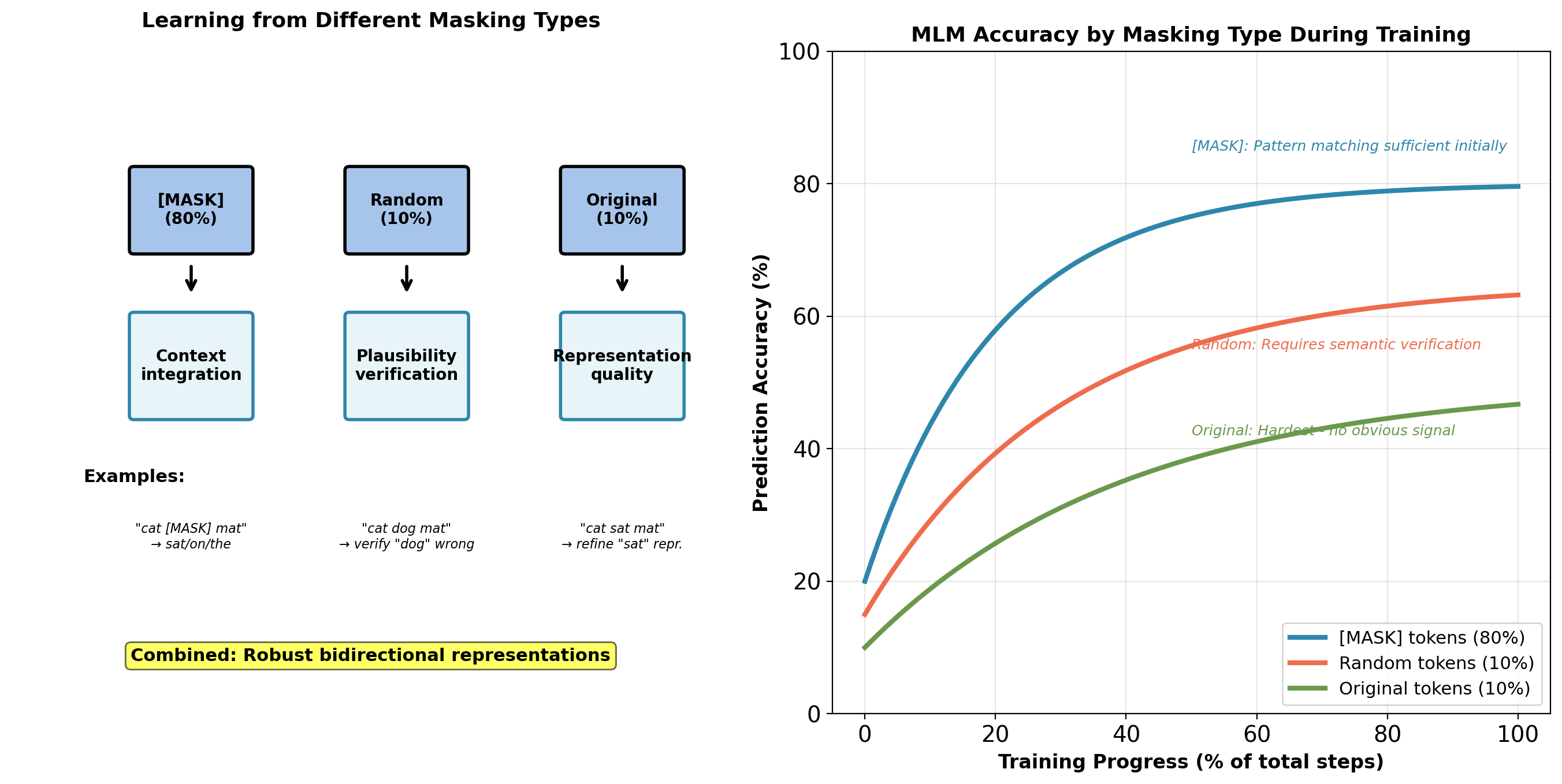
[MASK] tokens: Model learns fastest. Clear corruption signal.
Random tokens: Intermediate difficulty. Must verify semantic plausibility.
Original tokens: Hardest. No corruption signal, must predict from context alone.
This difficulty distribution forces model to develop robust representations.
MLM vs Autoregressive LM: Training Signal Comparison
GPT (Autoregressive):
\[\mathcal{L}_{\text{AR}} = -\sum_{i=1}^{T} \log P(x_i | x_{<i}; \theta)\]
Every position provides training signal. Context: Left-only (causal).
For T=512 sequence: 512 predictions, each using partial context.
BERT (Masked LM):
\[\mathcal{L}_{\text{MLM}} = -\sum_{i \in \mathcal{M}} \log P(x_i | \mathbf{x}_{\backslash \mathcal{M}}; \theta)\]
Only masked positions provide training signal. Context: Full bidirectional.
For T=512 sequence: 77 predictions (15%), each using full context.
Training signals per sequence:
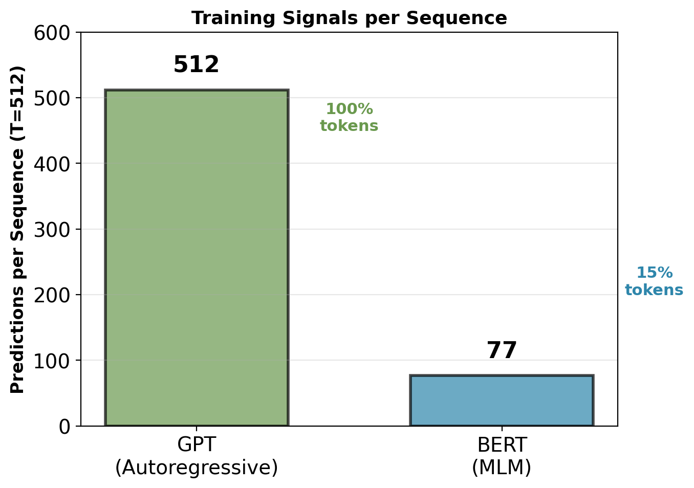
BERT uses 6.6× fewer tokens per sequence for supervision.
Requires more sequences to match GPT’s total training signals.
Context quality per prediction:
GPT at position i: - Context: \(x_1, \ldots, x_{i-1}\) (i-1 tokens) - Average context: T/2 ≈ 256 tokens - No future information
BERT at masked position i: - Context: All unmasked positions (≈437 tokens) - Full sequence context - Bidirectional information
Trade-off:
GPT: More training signals, less context per signal
BERT: Fewer training signals, richer context per signal
Empirical results (original papers):
GPT-1 training: 5B tokens, 30 days on 8 GPUs
BERT-base training: 3.3B tokens, 4 days on 64 TPUs
Different architectures and hardware, but BERT requires comparable data despite 6.6× fewer signals per sequence.
Bidirectional context compensates for fewer training signals.